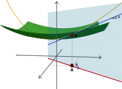
Calculus is the broad area of mathematics dealing with such topics as instantaneous rates of change, areas under curves, and sequences and series. Underlying all of these topics is the concept of a limit, which consists of analyzing the behavior of a function at points ever closer to a particular point, but without ever actually reaching that point. As a typical application of the methods of calculus, consider a moving car. It is possible to create a function describing the displacement of the car (where it is located in relation to a reference point) at any point in time as well as a function describing the velocity (speed and direction of movement) of the car at any point in time. If the car were traveling at a constant velocity, then algebra would be sufficient to determine the position of the car at any time; if the velocity is unknown but still constant, the position of the car could be used (along with the time) to find the velocity.
However, the velocity of a car cannot jump from zero to 35 miles per hour at the beginning of a trip, stay constant throughout, and then jump back to zero at the end. As the accelerator is pressed down, the velocity rises gradually, and usually not at a constant rate (i.e., the driver may push on the gas pedal harder at the beginning, in order to speed up). Describing such motion and finding velocities and distances at particular times cannot be done using methods taught in pre-calculus, whereas it is not only possible but straightforward with calculus.
Calculus has two basic applications: differential calculus and integral calculus. The simplest introduction to differential calculus involves an explicit series of numbers. Given the series (42, 43, 3, 18, 34), the differential of this series would be (1, -40, 15, 16). The new series is derived from the difference of successive numbers which gives rise to its name "differential". Rarely, if ever, are differentials used on an explicit series of numbers as done here. Instead, they are derived from a continuous function in a manner which is described later.
Integral calculus, like differential calculus, can also be introduced via series of numbers. Notice that in the previous example, the original series can almost be derived solely from its differential. Instead of taking the difference, however, integration involves taking the sum. Given the first number of the original series, 42 in this case, the rest of the original series can be derived by adding each successive number in its differential (42+1, 43-40, 3+15, 18+16). Note that knowledge of the first number in the original series is crucial in deriving the integral. As with differentials, integration is performed on continuous functions rather than explicit series of numbers, but the concept is still the same. Integral calculus allows us to calculate the area under a curve of almost any shape; in the car example, this enables you to find the displacement of the car based on the velocity curve. This is because the area under the curve is the total distance moved, as we will soon see.
Why learn calculus?
Calculus is essential for many areas of science and engineering. Both make heavy use of mathematical functions to describe and predict physical phenomena that are subject to continuous change, and this requires the use of calculus. Take our car example: if you want to design cars, you need to know how to calculate forces, velocities, accelerations, and positions. All require calculus. Calculus is also necessary to study the motion of gases and particles, the interaction of forces, and the transfer of energy. It is also useful in business whenever rates are involved. For example, equations involving interest or supply and demand curves are grounded in the language of calculus.
Calculus also provides important tools in understanding functions and has led to the development of new areas of mathematics including real and complex analysis, topology, and non-euclidean geometry.
Notwithstanding calculus' functional utility (pun intended), many non-scientists and non-engineers have chosen to study calculus just for the challenge of doing so. A smaller number of persons undertake such a challenge and then discover that calculus is beautiful in and of itself.
What is involved in learning calculus?
Learning calculus, like much of mathematics, involves two parts:
Understanding the concepts: You must be able to explain what it means when you take a derivative rather than merely apply the formulas for finding a derivative. Otherwise, you will have no idea whether or not your solution is correct. Drawing diagrams, for example, can help clarify abstract concepts.
Symbolic manipulation: Like other branches of mathematics, calculus is written in symbols that represent concepts. You will learn what these symbols mean and how to use them. A good working knowledge of trigonometry and algebra is a must, especially in integral calculus. Sometimes you will need to manipulate expressions into a usable form before it is possible to perform operations in calculus.
What you should know before using this text
There are some basic skills that you need before you can use this text. Continuing with our example of a moving car:
You will need to describe the motion of the car in symbols. This involves understanding functions.
You need to manipulate these functions. This involves algebra.
You need to translate symbols into graphs and vice versa. This involves understanding the graphing of functions.
It also helps (although it isn't necessarily essential) if you understand the functions used in trigonometry since these functions appear frequently in science.
Scope
The first four chapters of this textbook cover the topics taught in a typical high school or first year college course. The first chapter, Precalculus, reviews those aspects of functions most essential to the mastery of calculus. The second, Limits, introduces the concept of the limit process. It also discusses some applications of limits and proposes using limits to examine slope and area of functions. The next two chapters, Differentiation and Integration, apply limits to calculate derivatives and integrals. The Fundamental Theorem of Calculus is used, as are the essential formulas for computation of derivatives and integrals without resorting to the limit process. The third and fourth chapters include articles that apply the concepts previously learned to calculating volumes, and as other important formulas.
The remainder of the central calculus chapters cover topics taught in higher-level calculus topics: parametric and polar equations, sequences and series, multivariable calculus, and differential equations.
The final chapters cover the same material, using formal notation. They introduce the material at a much faster pace, and cover many more theorems than the other two sections. They assume knowledge of some set theory and set notation.
The purpose of this section is for readers to review important algebraic concepts. It is necessary to understand algebra in order to do calculus. If you are confident of your ability, you may skim through this section.
Rules of arithmetic and algebra
The following laws are true for all in whether these are numbers, variables, functions, or more complex expressions involving numbers, variable and/or functions.
Addition
Commutative Law: .
Associative Law: .
Additive Identity: .
Additive Inverse: .
Subtraction
Definition: .
Multiplication
Commutative law: .
Associative law: .
Multiplicative identity: .
Multiplicative inverse: , whenever
Distributive law: .
Division
Definition: , where r is the remainder of a when divided by b, and n is an integer.
Definition: , whenever .
Let's look at an example to see how these rules are used in practice.
(from the definition of division)
(from the associative law of multiplication)
(from multiplicative inverse)
(from multiplicative identity)
Of course, the above is much longer than simply cancelling out in both the numerator and denominator. However, it is important to know what the rules are so as to know when you are allowed to cancel. Occasionally people do the following, for instance, which is incorrect:
.
The correct simplification is
,
where the number cancels out in both the numerator and the denominator.
Interval notation
There are a few different ways that one can express with symbols a specific interval (all the numbers between two numbers). One way is with inequalities. If we wanted to denote the set of all numbers between, say, 2 and 4, we could write "all satisfying ". This excludes the endpoints 2 and 4 because we use instead of . If we wanted to include the endpoints, we would write "all satisfying ."
Another way to write these intervals would be with interval notation. If we wished to convey "all satisfying " we would write . This does not include the endpoints 2 and 4. If we wanted to include the endpoints we would write . If we wanted to include 2 and not 4 we would write ; if we wanted to exclude 2 and include 4, we would write .
Thus, we have the following table:
Endpoint conditions
Inequality notation
Interval notation
Including both 2 and 4
all satisfying
Not including 2 nor 4
all satisfying
Including 2 not 4
all satisfying
Including 4 not 2
all satisfying
In general, we have the following table, where .
Meaning
Interval Notation
Set Notation
All values greater than or equal to and less than or equal to
All values greater than and less than
All values greater than or equal to and less than
All values greater than and less than or equal to
All values greater than or equal to
All values greater than
All values less than or equal to
All values less than
All values
Note that and must always have an exclusive parenthesis rather than an inclusive bracket. This is because is not a number, and therefore cannot be in our set. is really just a symbol that makes things easier to write, like the intervals above.
The interval is called an open interval, and the interval is called a closed interval.
Intervals are sets and we can use set notation to show relations between values and intervals. If we want to say that a certain value is contained in an interval, we can use the symbol to denote this. For example, . Likewise, the symbol denotes that a certain element is not in an interval. For example .
Exponents and radicals
There are a few rules and properties involving exponents and radicals. As a definition we have that if is a positive integer then denotes factors of . That is,
If then we say that .
If is a negative integer then we say that .
If we have an exponent that is a fraction then we say that . In the expression , is called the index of the radical, the symbol is called the radical sign, and is called the radicand.
In addition to the previous definitions, the following rules apply:
Rule
Example
Simplifying expressions involving radicals
We will use the following conventions for simplifying expressions involving radicals:
Given the expression , write this as
No fractions under the radical sign
No radicals in the denominator
The radicand has no exponentiated factors with exponent greater than or equal to the index of the radical
Example: Simplify the expression
Using convention 1, we rewrite the given expression as
Notice that . Since the index of the radical is 2, our expression violates convention 4. We can reduce the exponent of the expression under the radical as follows:
is called the base and is called the exponent. Suppose we would like to solve for . We would like to apply an operation to both sides of the equation that will get rid of the base on the right-hand side of the equation. The operation we want is called the logarithm, or log for short, and it is defined as follows:
Definition: (Formal definition of a logarithm)
exactly if and , , and .
Logarithms are taken with respect to some base. What the equation is saying is that, when is the exponent of , the result will be .
Example
Example: Calculate
is the number such that . Well , so
Common bases for logarithms
When the base is not specified, is taken to mean the base 10 logarithm. Later on in our study of calculus we will commonly work with logarithms with base . In fact, the base logarithm comes up so often that it has its own name and symbol. It is called the natural logarithm, and its symbol is . In computer science the base 2 logarithm often comes up.
Properties of logarithms
Logarithmic addition and subtraction
Logarithms have the property that . To see why this is true, suppose that:
and
These assumptions imply that
and
Then by the properties of exponents
According to the definition of the logarithm
Similarly, the property that also hold true using the same method.
Historically, the development of logarithms was motivated by the usefulness of this fact for simplifying hand calculations by replacing tedious multiplication by table look-ups and addition.
Logarithmic powers and roots
Another useful property of logarithms is that . To see why, consider the expression . Let us assume that
By the definition of the logarithm
Now raise each side of the equation to the power and simplify to get
Now if you take the base log of both sides, you get
Solving for shows that
Similarly, the expression holds true using the same methods.
Converting between bases
Most scientific calculators have the and functions built in, which do not include logarithms with other bases. Consider how one might compute , where and are given known numbers, when we can only compute logarithms in some base . First, let us assume that
Then the definition of logarithm implies that
If we take the base log of each side, we get
Solving for , we find that
For example, if we only use base 10 to calculate , we get .
Identities of logarithms summary
A table is provided below for a summary of logarithmic identities.
Formula
Example
Product
Quotient
Power
Root
Change of base
Factoring and roots
Given the expression , one may ask "what are the values of that make this expression 0?" If we factor we obtain
.
If , then one of the factors on the right becomes zero. Therefore, the whole must be zero. So, by factoring we have discovered the values of that render the expression zero. These values are termed "roots." In general, given a quadratic polynomial that factors as
then we have that and are roots of the original polynomial.
A special case to be on the look out for is the difference of two squares, . In this case, we are always able to factor as
For example, consider . On initial inspection we would see that both and are squares of and , respectively. Applying the previous rule we have
The AC method
There is a way of simplifying the process of factoring using the AC method. Suppose that a quadratic polynomial has a formula of
If there are numbers and that satisfy both
and
Then, the result of factoring will be
The quadratic formula
The quadratic formula
Given any quadratic equation , all solutions of the equation are given by the quadratic formula:
Note that the value of will affect the number of real solutions of the equation.
If
Then
There are two real solutions to the equation
There is only one real solution to the equation
There are no real solutions to the equation
Example: Find all the roots of
Finding the roots is equivalent to solving the equation . Applying the quadratic formula with , we have:
The quadratic formula can also help with factoring, as the next example demonstrates.
Example: Factor the polynomial
We already know from the previous example that the polynomial has roots and . Our factorization will take the form
All we have to do is set this expression equal to our polynomial and solve for the unknown constant C:
You can see that solves the equation. So the factorization is
Vieta's formulae
Vieta's formulae relate the coefficients of a polynomial to sums and products of its roots. It is very convenient because under certain circumstances when the sums and products of the quadratic's roots are provided, one does not require to solve the whole quadratic polynomial.
Vieta's formulae in quadratic polynomials
Given any quadratic equation , The roots of the quadratic polynomial satisfy
Simplifying rational expressions
Consider the two polynomials
and
When we take the quotient of the two we obtain
The ratio of two polynomials is called a rational expression. Many times we would like to simplify such a beast. For example, say we are given . We may simplify this in the following way:
This is nice because we have obtained something we understand quite well, , from something we didn't.
Formulas of multiplication of polynomials
Here are some formulas that can be quite useful for solving polynomial problems:
Polynomial Long Division
Suppose we would like to divide one polynomial by another. The procedure is similar to long division of numbers and is illustrated in the following example:
Example
Divide (the dividend or numerator) by (the divisor or denominator)
Similar to long division of numbers, we set up our problem as follows:
First we have to answer the question, how many times does go into ? To find out, divide the leading term of the dividend by leading term of the divisor. So it goes in times. We record this above the leading term of the dividend:
, and we multiply by and write this below the dividend as follows:
Now we perform the subtraction, bringing down any terms in the dividend that aren't matched in our subtrahend:
Now we repeat, treating the bottom line as our new dividend:
In this case we have no remainder.
Application: Factoring Polynomials
We can use polynomial long division to factor a polynomial if we know one of the factors in advance. For example, suppose we have a polynomial and we know that is a root of . If we perform polynomial long division using P(x) as the dividend and as the divisor, we will obtain a polynomial such that , where the degree of is one less than the degree of .
Exercise
Use ^ to write exponents:
Application: Breaking up a rational function
Similar to the way one can convert an improper fraction into an integer plus a proper fraction, one can convert a rational function whose numerator has degree and whose denominator has degree with into a polynomial plus a rational function whose numerator has degree and denominator has degree with .
Suppose that divided by has quotient and remainder . That is
Dividing both sides by gives
will have degree less than .
Example
Write as a polynomial plus a rational function with numerator having degree less than the denominator.
Functions are everywhere, from a simple correlation between distance and time to complex heat waves. This chapter focuses on the fundamentals of functions: the definition, basic concepts, and other defining aspects. It is very concept-heavy, and expect a lot of reading and understanding. However, this is simply a review and an introduction on what is to come in future chapters.
Introduction
Definition of a function
An easy but vague way to understand functions is, to remember that a function is like a processor. It takes the input to change the output. Formally, a function f from a set X to a set Y is defined by a set G of ordered pairs (x, y) such that x ∈ X, y ∈ Y, and every element of X is the first component of exactly one ordered pair in G. In other words, for every x in X, there is exactly one element y such that the ordered pair (x, y) belongs to the set of pairs defining the function f. The set G is called the graph of the function. Formally speaking, it may be identified with the function, but this hides the usual interpretation of a function as a process. Therefore, in common usage, the function is generally distinguished from its graph.
Whenever one quantity uniquely determines the value of another quantity, we have a function. That is, the set uniquely determines the set . You can think of a function as a kind of machine. You feed the machine raw materials, and the machine changes the raw materials into a finished product.
A function in everyday life
Think about dropping a ball from a bridge. At each moment in time, the ball is a height above the ground. The height of the ball is a function of time. It was the job of physicists to come up with a formula for this function. This type of function is called real-valued since the "finished product" is a number (or, more specifically, a real number).
A function in everyday life (Preview of Multivariable Calculus)
Think about a wind storm. At different places, the wind can be blowing in different directions with different intensities. The direction and intensity of the wind can be thought of as a function of position. This is a function of two real variables (a location is described by two values - an and a ) which results in a vector (which is something that can be used to hold a direction and an intensity). These functions are studied in multivariable calculus (which is usually studied after a one year college level calculus course). This a vector-valued function of two real variables.
We will be looking at real-valued functions until studying multivariable calculus. Think of a real-valued function as an input-output machine; you give the function an input, and it gives you an output which is a number (more specifically, a real number). For example, the squaring function takes the input 4 and gives the output value 16. The same squaring function takes the input -1 and gives the output value 1.
This is an intuitive way to understand functions: a machine that makes the input go through a transformation into the output
Notation
Functions are used so much that there is a special notation for them. The notation is somewhat ambiguous, so familiarity with it is important in order to understand the intention of an equation or formula.
Though there are no strict rules for naming a function, it is standard practice to use the letters , , and to denote functions, and the variable to denote an independent variable. is used for both dependent and independent variables.
When discussing or working with a function , it's important to know not only the function, but also its independent variable . Thus, when referring to a function , you usually do not write , but instead . The function is now referred to as " of ". The name of the function is adjacent to the independent variable (in parentheses). This is useful for indicating the value of the function at a particular value of the independent variable. For instance, if
,
and if we want to use the value of for equal to , then we would substitute 2 for on both sides of the definition above and write
This notation is more informative than leaving off the independent variable and writing simply '' , but can be ambiguous since the parentheses next to can be misinterpreted as multiplication, . To make sure nobody is too confused, follow this procedure:
Define the function by equating it to some expression.
Give a sentence like the following: "At , the function is..."
Evaluate the function.
Description
There are many ways which people describe functions. In the examples above, a verbal description is given (the height of the ball above the earth as a function of time). Here is a list of ways to describe functions. The top three listed approaches to describing functions are the most popular.
A function is given a name (such as ) and a formula for the function is also given. For example, describes a function. We refer to the input as the argument of the function (or the independent variable), and to the output as the value of the function at the given argument.
A function is described using an equation and two variables. One variable is for the input of the function and one is for the output of the function. The variable for the input is called the independent variable. The variable for the output is called the dependent variable. For example, describes a function. The dependent variable appears by itself on the left hand side of equal sign.
A verbal description of the function.
When a function is given a name (like in number 1 above), the name of the function is usually a single letter of the alphabet (such as or ). Some functions whose names are multiple letters (like the sine function )
Plugging a value into a function
If we write , then we know that
The function is a function of .
To evaluate the function at a certain number, replace the with that number.
Replacing with that number in the right side of the function will produce the function's output for that certain input.
In English, the definition of is interpreted, "Given a number, will return two more than the triple of that number."
How would we know the value of the function at 3?
We would have the following three thoughts:
and we would write
.
The value of at 3 is 11.
Note that means the value of the dependent variable when takes on the value of 3. So we see that the number 11 is the output of the function when we give the number 3 as the input. People often summarize the work above by writing "the value of at three is eleven", or simply " of three equals eleven".
Basic concepts of functions
The formal definition of a function states that a function is actually a mapping that associates the elements of one set called the domain of the function, , with the elements of another set called the range of the function, . For each value we select from the domain of the function, there exists exactly one corresponding element in the range of the function. The definition of the function tells us which element in the range corresponds to the element we picked from the domain. An example of how is given below.
Let function for all . For what value of gives ?
In mathematics, it is important to notice any repetition. If something seems to repeat, keep a note of that in the back of your mind somewhere.
Here, notice that and . Because is equal to two different things, it must be the case that the other side of the equal sign to is equal to the other. This property is known as the transitive property and could thus make the following equation below true:
Next, simplify — make your life easier rather than harder. In this instance, since has as a like-term, and the two terms are fractions added to the other, put it over a common denominator and simplify. Similar, since is a mixed fraction, .
Multiply both sides by the reciprocal of the coefficient of , from both sides by multiplying by it.
or.
The value of that makes is ..
Classically, the element picked from the domain is pictured as something that is fed into the function and the corresponding element in the range is pictured as the output. Since we "pick" the element in the domain whose corresponding element in the range we want to find, we have control over what element we pick and hence this element is also known as the "independent variable". The element mapped in the range is beyond our control and is "mapped to" by the function. This element is hence also known as the "dependent variable", for it depends on which independent variable we pick. Since the elementary idea of functions is better understood from the classical viewpoint, we shall use it hereafter. However, it is still important to remember the correct definition of functions at all times.
Basic types of transformation
To make it simple, for the function , all of the possible values constitute the domain, and all of the values ( on the x-y plane) constitute the range. To put it in more formal terms, a function is a mapping of some element , called the domain, to exactly one element , called the range, such that . The image below should help explain the modern definition of a function:
is the domain of the function while is the range. This transformation from set to is an example of one-to-one function.
A function is considered one-to-one if an element from domain of function , leads to exactly one element from range of the function. By definition, since only one element is mapped by function from some element , implies that there exists only one element from the mapping. Therefore, there exists a one-to-one function because it complies with the definition of a function. This definition is similar to Figure 1.
A function is considered many-to-one if some elements from domain of function maps to exactly one element from range of the function. Since some elements must map onto exactly one element , must be compliant with the definition of a function. Therefore, there exists a many-to-one function.
A function is considered one-to-many if exactly one element from domain of function maps to some elements from range of the function. If some element maps onto many distinct elements , then is non-functional since there exists many distinct elements . Given many-to-one is non-compliant to the definition of a function, there exists no function that is one-to-many.
The modern definition describes a function sufficiently such that it helps us determine whether some new type of "function" is indeed one. Now that each case is defined above, you can now prove whether functions are one of these function cases. Here is an example problem:
Given: , where and are constant and . Prove: function is one-to-one.
Notice that the only changing element in the function is . To prove a function is one-to-one by applying the definition may be impossible because although two random elements of domain set may not be many-to-one, there may be some elements that may make the function many-to-one. To account for this possibility, we must prove that it is impossible to have some result like that.
Assume there exists two distinct elements that will result in . This would make the function many-to-one. In consequence,
Subtract from both sides of the equation.
Subtract from both sides of the equation.
Factor from both terms to the left of the equation.
Multiply to both sides of the equation.
Add to both sides of the equation.
Notice that . However, this is impossible because and are distinct. Ergo, . No two distinct inputs can give the same output. Therefore, the function must be one-to-one.
Basic concepts
The domain is all the elements in set that can be mapped to the elements in set . The range is those elements in set which are mapped with the domain. The codomain is all the elements in set .
There are a few more important ideas to learn from the modern definition of the function, and it comes from knowing the difference between domain, range, and codomain. We already discussed some of these, yet knowing about sets adds a new definition for each of the following ideas. Therefore, let us discuss these based on these new ideas. Let and be a set. If we were to combine these two sets, it would be defined as the cartesian cross product. The subset of this product is the function. The below definitions are a little confusing. The best way to interpret these is to draw an image. To the right of these definitions is the image that corresponds to it.
Definition of domain, range, and codomain of a function
The domain is defined to be a set
with all elements mapping to at least one unique .
The set of elements in is the range of the function mapping in the cartesian cross product, whereby the set of all elements maps to some element .
The codomain is the set , where it is not necessarily the case that all elements was mapped by some .
Note that the codomain is not as important as the other two concepts.
Take for example:
The domain of the function is the interval from -1 to 1
Because of the square root, the content in the square root should be strictly not smaller than 0.
Thus the domain is
The range of the function is the interval from 0 to 1
Correspondingly, the range will be
Other types of transformation
There is one more final aspect that needs to be defined. We already have a good idea of what makes a mapping a function (e.g. it cannot be one-to-many). However, three more definitions that you will often hear will be necessary to talk about: injective, surjective, bijective.
The function mapping on the left is an example of an injective function because it is one-to-one. However, it is not surjective because the range and the codomain are not the same.
A function is injective if it is one-to-one.
A function is surjective if it is "onto." That is, the mapping has as the range of the function, where the codomain and the range of the function are the same.
A function is bijective if it is both surjective and injective.
Again, the above definitions are often very confusing. Again, another image is provided to the right of the bullet points. Along with that, another example is also provided. Let us analyze the function .
Given: , where is constant and . Prove: function is non-surjective and non-injective.
Notice that the only changing element in the function is . Let us check to see the conditions of this function.
Is it injective? Let , and solve for . First, divide by .
Then take the square root of . By definition, , so
Notice, however, what we learned from the above manipulation. As a result of solving for , we found that there are two solutions for . However, this resulted in two different values from . This means that for some individual that gives , there are two different inputs that result in the same value. Because when , this is by definition non-injective.
Is it surjective? As a natural consequence of what we learned about inputs, let us determine the range of the function. After all, the only way to determine if something is surjective is to see if the range applies to all real numbers. A good way to determine this is by finding a pattern involving our domains. Let us say we input a negative number for the domain: . This seemingly trivial exercise tells us that negative numbers give us non-negative numbers for our range. This is huge information! For , the function always results for our range. For the set , we have elements in that set that have no mappings from the set . As such, is the codomain of set . Therefore, this function is non-surjective!
This is an example of an expression which fails the vertical line test.
Tests for equations
The vertical line test
The vertical line test is a systematic test to find out if an equation involving and can serve as a function (with the independent variable and the dependent variable). Simply graph the equation and draw a vertical line through each point of the -axis. If any vertical line ever touches the graph at more than one point, then the equation is not a function; if the line always touches at most one point of the graph, then the equation is a function.
The circle, on the right, is not a function because the vertical line intercepts two points on the graph when .
The horizontal line and the algebraic 1-1 test
Similarly, the horizontal line test, though does not test if an equation is a function, tests if a function is injective (one-to-one). If any horizontal line ever touches the graph at more than one point, then the function is not one-to-one; if the line always touches at most one point on the graph, then the function is one-to-one.
The algebraic 1-1 test is the non-geometric way to see if a function is one-to-one. The basic concept is that:
Assume there is a function . If:
, and , then
function is one-to-one.
Here is an example: prove that is injective.
Since the notation is the notation for a function, the equation is a function. So we only need to prove that it is injective. Let and be the inputs of the function and that . Thus,
So, the result is , proving that the function is injective.
Another example is proving that is not injective.
Using the same method, one can find that , which is not . So, the function is not injective.
Remarks
The following arise as a direct consequence of the definition of functions:
By definition, for each "input" a function returns only one "output", corresponding to that input. While the same output may correspond to more than one input, one input cannot correspond to more than one output. This is expressed graphically as the vertical line test: a line drawn parallel to the axis of the dependent variable (normally vertical) will intersect the graph of a function only once. However, a line drawn parallel to the axis of the independent variable (normally horizontal) may intersect the graph of a function as many times as it likes. Equivalently, this has an algebraic (or formula-based) interpretation. We can always say if , then , but if we only know that then we can't be sure that .
Each function has a set of values, the function's domain, which it can accept as input. Perhaps this set is all positive real numbers; perhaps it is the set {pork, mutton, beef}. This set must be implicitly/explicitly defined in the definition of the function. You cannot feed the function an element that isn't in the domain, as the function is not defined for that input element.
Each function has a set of values, the function's range, which it can output. This may be the set of real numbers. It may be the set of positive integers or even the set {0,1}. This set, too, must be implicitly/explicitly defined in the definition of the function.
Functions are an important foundation of mathematics. This modern interpretation is a result of the hard work of the mathematicians of history. It was not until recently that the definition of the relation was introduced by René Descartes in Geometry (1637). Nearly a century later, the standard notation () was first introduced by Leonhard Euler in Introductio in Analysin Infinitorum and Institutiones Calculi Differentialis. The term function was also a new innovation during Euler's time as well, being introduced Gottfried Wilhelm Leibniz in a 1673 letter "to describe a quantity related to points of a curve, such as a coordinate or curve's slope." Finally, the modern definition of the function being the relation among sets was first introduced in 1908 by Godfrey Harold Hardy where there is a relation between two variables and such that "to some values of at any rate correspond values of ." For the person that wants to learn more about the history of the function, go to History of functions.
Important functions
The functions listed below are essential to calculus. This section only serves as a review and scratches the surface of those functions. If there are any questions about those functions, please review the materials related to those functions before continuing. More about graphing will be explained in Chapter 1.4
Polynomials
Polynomial functions are the most common and most convenient functions in the world of calculus. Their frequent appearances and their applications on computer calculations have made them important.
Definition of a polynomial function
A polynomial in a single indeterminate x can always be written (or rewritten) in the form:
To be more concise, it can also be written in the summation form:
Constant
Two linear functions are shown on the image. One is and the other is
When , the polynomial can be rewritten into the following function:
, where is a constant.
The graph of this function is a horizontal line passing the point .
Linear
When , the polynomial can be rewritten into
, where are constants.
The graph of this function is a straight line passing the point and , and the slope of this function is .
This is the graph of a quadratic function.
Quadratic
When , the polynomial can be rewritten into
, where are constants.
The graph of this function is a parabola, like the trajectory of a basketball thrown into the hoop.
If there are questions about the quadratic formula and other basic polynomial concepts, please review the respective chapters in Algebra.
Trigonometric
Trigonometric functions are also very important because it can connect algebra and geometry. Trigonometric functions are explained in detail here due to its importance and difficulty.
The curve on the left is an exponential function while the curve on the right is a logarithmic one
Exponential and Logarithmic
Exponential and logarithmic functions have a unique identity when calculating the derivatives, so this is a great time to review those functions.
Definition for exponential and logarithmic functions
The exponential function is defined as:
, where is a constant.
while the logarithmic function is defined as:
, where is a constant.
A special number will be frequently seen in those functions: the Euler's constant, also known as the base of the natural logarithm. Notated as , it is defined as .
Signum
The Signum (sign) function is simply defined as
Properties of functions
Sometimes, a lot of function manipulations cannot be achieved without some help from basic properties of functions.
Domain and range
This concept is discussed above.
Growth
Although it seems obvious to spot a function increasing or decreasing, without the help of graphing software, we need a mathematical way to spot whether the function is increasing or decreasing, or else our human minds cannot immediately comprehend the huge amount of information.
Assume a function with inputs , and that , , and at all times.
If for all and , , then
is increasing in
If for all and , , then
is decreasing in
Example: In which intervals is increasing?
Firstly, the domain is important. Because the denominator cannot be 0, the domain for this function is
In , the growth of the function is:
Let and
Thus,
both
and
So,
is decreasing in
In
Let and
Thus,
both
However, the sign of in cannot be determined. It can only be determined in .
In
and
In
As a result,
is decreasing in and increasing in .
In
Let and
Thus,
both
So,
is increasing in .
Therefore, the intervals in which the function is increasing are .
After learning derivatives, there will be more ways to determine the growth of a function.
Parity
The properties odd and even are associated with symmetry. While even functions have a symmetry about the -axis, odd functions are symmetric about the origin. In mathematical terms:
A function is even when
A function is odd when
Example: Prove that is an even function.
is an even function
Manipulating functions
Addition, Subtraction, Multiplication and Division of functions
For two real-valued functions, we can add the functions, multiply the functions,
raised to a power, etc.
Example: Adding, subtracting, multiplying and dividing functions which do not have a name
If we add the functions and , we obtain .
If we subtract from , we obtain . We can also write this as .
If we multiply the function and the function , we obtain . We can also write this as .
If we divide the function by the function , we obtain .
If a math problem wants you to add two functions and , there are two ways that the problem will likely be worded:
If you are told that , that , that and asked about , then you are being asked to add two functions. Your answer would be .
If you are told that , that and you are asked about , then you are being asked to add two functions. The addition of and is called . Your answer would be .
Similar statements can be made for subtraction, multiplication and division.
Example: Adding, subtracting, multiplying and dividing functions which do have a name
Let and: . Let's add, subtract, multiply and divide.
,
,
,
.
Composition of functions
We begin with a fun (and not too complicated) application of composition of functions before we talk about what composition of functions is.
Example: Dropping a ball
If we drop a ball from a bridge which is 20 meters above the ground, then the height of our ball above the earth is a function of time. The physicists tell us that if we measure time in seconds and distance in meters, then the formula for height in terms of time is . Suppose we are tracking the ball with a camera and always want the ball to be in the center of our picture. Suppose we have The angle will depend upon the height of the ball above the ground and the height above the ground depends upon time. So the angle will depend upon time. This can be written as . We replace with what it is equal to. This is the essence of composition.
Composition of functions is another way to combine functions which is different from addition,
subtraction, multiplication or division.
The value of a function depends upon the value of another variable ; however, that variable could be equal to another function , so its value depends on the value of a third variable. If this is the case, then the first variable is a function of the third variable; this function () is called the composition of the other two functions ( and ).
Example: Composing two functions
Let and: . The composition of with is read as either "f composed with g" or "f of g of x."
Let
Then
.
Sometimes a math problem asks you compute
when they want you to compute ,
Here, is the composition of and and we write . Note that composition is not commutative:
, and
so .
Composition of functions is very common, mainly because functions themselves are common. For instance, squaring and sine are both functions:
Thus, the expression is a composition of functions:
(Note that this is not the same as .)
Since the function sine equals if ,
.
Since the function square equals if ,
.
Transformations
Transformations are a type of function manipulation that are very common. They consist of multiplying, dividing, adding or subtracting constants to either the input or the output. Multiplying by a constant is called dilation and adding a constant is called translation. Here are a few examples:
Dilation
Translation
Dilation
Translation
Examples of horizontal and vertical translationsExamples of horizontal and vertical dilations
Translations and dilations can be either horizontal or vertical. Examples of both vertical and horizontal translations can be seen at right. The red graphs represent functions in their 'original' state, the solid blue graphs have been translated (shifted) horizontally, and the dashed graphs have been translated vertically.
Dilations are demonstrated in a similar fashion. The function
has had its input doubled. One way to think about this is that now any change in the input will be doubled. If I add one to , I add two to the input of , so it will now change twice as quickly. Thus, this is a horizontal dilation by because the distance to the -axis has been halved. A vertical dilation, such as
is slightly more straightforward. In this case, you double the output of the function. The output represents the distance from the -axis, so in effect, you have made the graph of the function 'taller'. Here are a few basic examples where is any positive constant:
Original graph
Rotation about origin
Horizontal translation by units left
Horizontal translation by units right
Horizontal dilation by a factor of
Vertical dilation by a factor of
Vertical translation by units down
Vertical translation by units up
Reflection about -axis
Reflection about -axis
Inverse functions
We call the inverse function of if, for all :
A function has an inverse function if and only if is one-to-one. For example, the inverse of is . The function has no inverse because it is not injective. Similarly, the inverse functions of trigonometric functions have to undergo transformations and limitations to be considered as valid functions.
Notation
The inverse function of is denoted as . Thus, is defined as the function that follows this rule
To determine when given a function , substitute for and substitute for . Then solve for , provided that it is also a function.
Example: Given , find .
Substitute for and substitute for . Then solve for :
To check your work, confirm that :
If isn't one-to-one, then, as we said before, it doesn't have an inverse. Then this method will fail.
Example: Given , find .
Substitute for and substitute for . Then solve for :
Since there are two possibilities for , it's not a function. Thus doesn't have an inverse. Of course, we could also have found this out from the graph by applying the Horizontal Line Test. It's useful, though, to have lots of ways to solve a problem, since in a specific case some of them might be very difficult while others might be easy. For example, we might only know an algebraic expression for but not a graph.
<h1>Failed to match page to section number. Check your argument; if correct, consider updating Template:Calculus/map page. Graphing linear functions</h1>
Graph of y=2x
It is sometimes difficult to understand the behavior of a function given only its definition; a visual representation or graph can be very helpful. A graph is a set of points in the Cartesian plane, where each point indicates that . In other words, a graph uses the position of a point in one direction (the vertical-axis or -axis) to indicate the value of for a position of the point in the other direction (the horizontal-axis or -axis).
Functions may be graphed by finding the value of for various and plotting the points in a Cartesian plane. For the functions that you will deal with, the parts of the function between the points can generally be approximated by drawing a line or curve between the points. Extending the function beyond the set of points is also possible, but becomes increasingly inaccurate.
Linear functions
Graphing linear functions are easy to understand and do. Because we know that two points can form a line, only two points are needed for us to graph a linear function if those two points are on the function. Oppositely, we can write down the equation of a linear function if we only know two points that are on the function.
The following section mainly talks about different forms of linear function notations so that you can easily identify or graph the function.
Introduction
Plotting points like this is laborious. Fortunately, many functions' graphs fall into general patterns. For a simple case, consider functions of the form
The graph of is a single line, passing through the point with slope 3. Thus, after plotting the point, a straightedge may be used to draw the graph. This type of function is called linear and there are a few different ways to present a function of this type.
Slope
The slope is the backbone of linear functions because it shows how much the output of a function changes when the input changes. For example, if the slope of a function is 2, then it means when the input of a function increases by 1 unit, the output of the function increases by 2 units. Now, let's look at a more mathematical example.
Consider this function: . What does the number mean?
It means that when increases by 1, decreases by 5.
Using mathematical terms:
It is easy to calculate the slope because the slope is like the speed of a vehicle. If we divide the change in distance and the corresponding change in time, we get the speed. Similarly, if we divide the change in over the corresponding change in , we get the slope.
If given two points, and , we may then compute the slope of the line that passes through these two points. Remember, the slope is determined as "rise over run." That is, the slope is the change in -values divided by the change in -values. In symbols:
Slope in a linear function
If two points and on a linear function, then the slope of the linear function is
Interestingly, there is a subtle relationship between the slope and the angle between the graph of the function and the positive -axis, . The relationship is:
It is an obvious relationship, but it can be ignored relatively easily.
Slope-intercept form
This is a linear function notated in the slope-intercept form. The slope here is instead of .
When we see a function presented as
we call this presentation the slope-intercept form. This is because, not surprisingly, this way of writing a linear function involves the slope, , and the -intercept, .
Example 1: Graph the function .
The slope of the function is 3, and it intercepts the -axis at point . In order to graph the function, we need another point. Since the slope of the function is 3, then
Knowing that the function goes through points , the function can be easily graphed.
Example 2: Now, consider another unknown linear function that goes through points . What is the equation for this function?
The slope can be calculate with the formula mentioned above.
And since the -axis interception is , we can know that
Thus, the equation of this linear function should be
Point-slope form
If someone walks up to you and gives you one point and a slope, you can draw one line and only one line that goes through that point and has that slope. Said differently, a point and a slope uniquely determine a line. So, if given a point and a slope , we present the graph as
We call this presentation the point-slope form. The point-slope and slope-intercept form are essentially the same. In the point-slope form we can use any point the graph passes through. Where as, in the slope-intercept form, we use the -intercept, that is the point . The point-slope form is very important. Although it is not used as frequently as its counterpart the slope-intercept form, the concept of knowing a point and drawing the line in the direction of the slope will be encountered when we go into vector equations for lines and planes in future chapters.
Example 1: If a linear function goes through points , what is the equation for this function?
The slope is:
Since we know two points, the following answers are all correct
The two-point form is another form to write the equation for a linear function. It is similar to the point-slope form. Given points and , we have the equation
This presentation is in the two-point form. It is essentially the same as the point-slope form except we substitute the expression for . However, this expression is not widely used in mathematics because in most situations, and are known coordinates. It would be redundant to write down a bulky instead of a simple expression of the slope.
Intercept form
The intercept form looks like this:
By writing the function in the intercept form, we can quickly determine the -axis intercepts.
-axis intercept:
-axis intercept:
When we discuss planes in 3D space, this form will be quite useful to determine the -axis intercepts.
Quadratic functions
To graph a quadratic function, there is the simple but work-heavy way, and there is the complicated but clever way. The simple way is to substitute the independent variable with various numbers and calculate the output . After some substitutions, plot those and connect those points with a curve. The complicated way is to find special points, such as intercepts and the vertex, and plot it out. The following section is a guide to find those special points, which will be useful in later chapters.
Actually, there is a third way, which we will discuss in Chapter 1.6.
Standard form
Quadratic functions are functions that look like this
, where are constants
The constant determines the concavity of the function: if , concaves up; if , concaves down.
The constant is the -coordinate of the -axis interception. In other words, this function goes through point .
Vertex form
The vertex form has its advantages over the standard form. While the standard form can determine the concavity and the -axis interception, the vertex form can, as the name suggests, determine the vertex of the function. The vertex of a quadratic function is the highest/lowest point on the graph of a function, depending on the concavity. If , the vertex is the lowest point on the graph; if , the vertex is the highest point on the graph.
The vertex form looks like this:
, where are constants
The vertex of this function is because when , . If , is the absolute minimum value that the function can achieve. If , is the absolute maximum value that the function can achieve.
Any standard form can be converted into the vertex form. The vertex form with constants looks like this
, where are constants in the standard form
Factored form
The factored form can determine the -axis intercepts because the factored form looks like this
, where are constants and are solutions for the equation
Thus, it can be determined that the function passes through points .
However, only certain functions can be written in this form. If the quadratic function does not have -axis intercept, it is impossible to write it in the factored form.
Example 1: What is the vertex of this function?
The equation can be transformed into the vertex form very easily
Thus, the vertex is .
Example 2: The image on the right is a quadratic function. Describe the meaning of the colored texts, which are important properties of a quadratic function.
This is the equation for the quadratic function. In this case, , .
Since there are two -axis intercepts, we can find that .
Points
This is an image of a quadratic function with key values.
These are the coordinates for the two -axis intercepts.
Knowing the coordinates, the function can be written in its factored form:
If you have difficulties deriving the quadratic formula or understanding the expression , see Quadratic function.
Point
This is the vertex for the quadratic function. Because , the vertex is the lowest point on the graph.
Since the vertex is known, we can write the function in the vertex form:
Although this does not look like the equation we've just discussed earlier, note that .
Line
The graph of the function is symmetric about this line. In other words,
Point and line will be discussed in the next chapter (1.6). They are the focus and the directrix respectively.
If you can skillfully and quickly determine those special points, graphing quadratic functions will be less torturing.
Exponential and Logarithmic functions
Exponential and logarithmic functions are inverse functions with each other. Take the exponential function for example. The inverse function of , , is
which is a logarithmic function.
Since geometrically, the graph of the inverse function is flipping the graph of the original function over line , we only need to know how to graph one of those functions.
Limits, the first step into calculus, explain the complex nature of the subject. It is used to define the process of derivation and integration. It is also used in other circumstances to intuitively demonstrate the process of "approaching".
Introduction
Intuitive Look into Limits
The limit is one of the greatest tools in the hands of any mathematician. We will give the limit an approach. Because mathematics came only due to approaches... remember?!
We designate limit in the form:
This is read as "The limit of of as approaches ". This is an important thing to remember, it is basic notation which is accepted by the world.
We'll take up later the question of how we can determine whether a limit exists for at and, if so, what it is. For now, we'll look at it from an intuitive standpoint.
Let's say that the function that we're interested in is , and that we're interested in its limit as approaches . Using the above notation, we can write the limit that we're interested in as follows:
One way to try to evaluate what this limit is would be to choose values near 2, compute for each, and see what happens as they get closer to 2. There are two ways to approach values near 2. One is to approach from below, and the other is to approach from above:
1.7
1.8
1.9
1.95
1.99
1.999
2.89
3.24
3.61
3.8025
3.9601
3.996001
The table above is the case from below.
2.3
2.2
2.1
2.05
2.01
2.001
5.29
4.84
4.41
4.2025
4.0401
4.004001
The table above is the case from above.
We can see from the tables that as grows closer and closer to 2, seems to get closer and closer to 4, regardless of whether approaches 2 from above or from below. For this reason, we feel reasonably confident that the limit of as approaches 2 is 4, or, written in limit notation,
We could have also just substituted 2 into and evaluated: . However, this will not work with all limits.
Now let's look at another example. Suppose we're interested in the behavior of the function as approaches 2. Here's the limit in limit notation:
Just as before, we can compute function values as approaches 2 from below and from above. Here's a table, approaching from below:
1.7
1.8
1.9
1.95
1.99
1.999
-3.333
-5
-10
-20
-100
-1000
And here from above:
2.3
2.2
2.1
2.05
2.01
2.001
3.333
5
10
20
100
1000
In this case, the function doesn't seem to be approaching a single value as approaches 2, but instead becomes an extremely large positive or negative number (depending on the direction of approach). Well, one says such a limit does not exist because no finite number is approached. This arises the concept of infinity: an undefined quantity and the limit is also called infinite limit or limit without a bound.
Note that we cannot just substitute 2 into and evaluate as we could with the first example, since we would be dividing by 0.
Both of these examples may seem trivial, but consider the following function:
This function is the same as
Note that these functions are really completely identical; not just "almost the same," but actually, in terms of the definition of a function, completely the same; they give exactly the same output for every input.
In elementary algebra, a typical approach is to simply say that we can cancel the term , and then we have the function . However, that would be inaccurate; the function that we have now is not really the same as the one we started with, because it is defined when , and our original function was specifically not defined when . This may seem like a minor point, but from making this kind of assumptions we can easily derive absurd results, such that (see Mathematical Fallacy § All numbers equal all other numbers in Wikipedia for a complete example). Even without calculus we can avoid this error by stating that:
In calculus, we can introduce a more intuitive and also correct way of looking at this type of function. What we want is to be able to say that, although the function isn't defined when , it works almost as if it was. It may not get there, but it gets really, really close. For instance, . The only question that we have is: what do we mean by "close"?
Informal Definition of a Limit
As the precise definition of a limit is a bit technical, it is easier to start with an informal definition; we'll explain the formal definition later.
We suppose that a function is defined for near (but we do not require that it be defined when ).
Informal definition of a limit
We call the limit of as approaches if becomes close to when is close (but not equal) to , and if there is no other value with the same property.
When this holds we write
or
Notice that the definition of a limit is not concerned with the value of when (which may exist or may not). All we care about are the values of when is close to , on either the left or the right (i.e. less or greater).
Limit can also be understood as: is infinitely approaching to but never equals to , just like the function , which infinitely approaches to but never equals .
Basics
Rules and Identities
Now that we have defined, informally, what a limit is, we will list some rules that are useful for working with and computing limits. You will be able to prove all these once we formally define the fundamental concept of the limit of a function.
First, the constant rule states that if (that is, is constant for all ) then the limit as approaches must be equal to . In other words
Constant Rule for Limits
If and are constants then .
Example:
Second, the identity rule states that if (that is, just gives back whatever number you put in) then the limit of as approaches is equal to . That is,
Identity Rule for Limits
If is a constant then .
Example:
The next few rules tell us how, given the values of some limits, to compute others.
Operational Identities for Limits
Suppose that and and that is constant. Then
Notice that in the last rule we need to require that is not equal to 0 (otherwise we would be dividing by zero which is an undefined operation).
These rules are known as identities; they are the scalar product, sum, difference, product, and quotient rules for limits. (A scalar is a constant, and, when you multiply a function by a constant, we say that you are performing scalar multiplication.)
Using these rules we can deduce another. Namely, using the rule for products many times we get that
for a positive integer .
This is called the power rule.
As a result, we can safely say that all limits for polynomial functions can be deduced into several limits that satisfy the identity rule and thus easier to compute.
Example 1
Find the limit .
We need to simplify the problem, since we have no rules about this expression by itself. We know from the identity rule above that . By the power rule, . Lastly, by the scalar multiplication rule, we get .
Example 2
Find the limit .
To do this informally, we split up the expression, once again, into its components. As above, .
Also and . Adding these together gives
.
Example 3
Find the limit .
From the previous example the limit of the numerator is . The limit of the denominator is
As the limit of the denominator is not equal to zero we can divide. This gives
.
Example 4
Find the limit .
We apply the same process here as we did in the previous set of examples;
.
We can evaluate each of these;
Thus, the answer is .
Example 5
Find the limit .
In this example, evaluating the result directly will result in a division by 0. While you can determine the answer experimentally, a mathematical solution is possible as well.
First, the numerator is a polynomial that may be factored:
Now, you can divide both the numerator and denominator by :
Remember that the limit is a method to determine the approaching value of a function instead of the value of the function itself. So, though the function is undefined at , the value of the function is approaching to when
Example 6
Find the limit .
To evaluate this seemingly complex limit, we will need to recall some sine and cosine identities (see Chapter 1.3). We will also have to use two new facts. First, if is a trigonometric function (that is, one of sine, cosine, tangent, cotangent, secant and cosecant functions), and is defined at , then .
Second, . This can be proved using squeeze theorem. Note that L'Hopital's rule is not allowed to be used to evaluate this limit because it causes circular reasoning,
in the sense that differentiating .requires this limit to equal one, which is exactly the equation that is being proven.
Method 1 (before learning L'Hôpital's rule):
To evaluate the limit, recognize that can be multiplied by to obtain which, by our trig identities, is . So, multiply the top and bottom by . (This is allowed because it is identical to multiplying by one.) This is a standard trick for evaluating limits of fractions; multiply the numerator and the denominator by a carefully chosen expression which will make the expression simplify somehow. In this case, we should end up with:
.
Our next step should be to break this up into by the product rule. As mentioned above, .
Next, .
Thus, by multiplying these two results, we obtain 0.
Note that we also cannot apply L'Hospital's rule to evaluate this limit because it causes circular reasoning.
We will now present an amazingly useful result, even though we cannot prove it yet. We can find the limit at of any polynomial or rational function, as long as that rational function is defined at (so we are not dividing by 0). That is, must be in the domain of the function.
Limits of Polynomials and Rational functions
If is a polynomial or rational function that is defined at then
We already learned this for trigonometric functions, so we see that it is easy to find limits of polynomial, rational or trigonometric functions wherever they are defined. In fact, this is true even for combinations of these functions; thus, for example, .
The Squeeze Theorem
Graph showing (blue) being squeezed between (red) and (green)
The Squeeze Theorem is very important in calculus, where it is typically used to find the limit of a function by comparison with two other functions whose limits are known.
It is called the Squeeze Theorem because it refers to a function whose values are squeezed between the values of two other functions and , both of which have the same limit . If the value of is trapped between the values of the two functions and , the values of must also approach .
Expressed more precisely:
Theorem: (Squeeze Theorem)
Suppose that holds for all in some open interval containing .
If ,
Then .
Plot of for
Example: Compute .
Since we know that
Multiplying into the inequality yields
Now we apply the squeeze theorem
Since ,
Finding Limits
Now, we will discuss how, in practice, to find limits. First, if the function can be built out of rational, trigonometric, logarithmic, or exponential functions, then if a number is in the domain of the function, then the limit at is simply the value of the function at :
when can be built out of rational, trigonometric, logarithmic, or exponential functions and the Domain of
If is not in the domain of the function, then in many cases (as with rational functions) the domain of the function includes all the points near , but not itself. An example would be if we wanted to find , where the domain includes all numbers besides 0.
In that case, in order to find we want to find a function similar to , except with the hole at filled in. The limits of and will be the same, as can be seen from the definition of a limit. By definition, the limit depends on only at the points where is close to but not equal to it, so the limit at does not depend on the value of the function at . Therefore, if , also. And since the domain of our new function includes , we can now (assuming is still built out of rational, trigonometric, logarithmic and exponential functions) just evaluate it at as before. Thus we have .
In our example, this is easy; canceling the 's gives , which equals at all points except 0. Thus, we have . In general, when computing limits of rational functions, it's a good idea to look for common factors in the numerator and denominator.
Specific DNE Situations
Note that the limit might not exist at all (DNE means "does not exist"). There are a number of ways in which this can occur:
"Gap"
There is a gap (not just a single point) where the function is not defined. As an example, in
does not exist when . There is no way to "approach" the middle of the graph. Note that the function also has no limit at the endpoints of the two curves generated (at and ). For the limit to exist, the point must be approachable from both the left and the right.
Note also that there is no limit at a totally isolated point on a graph.
Jump discontinuity.
"Jump"
If the graph suddenly jumps to a different level, there is no limit at the point of the jump. For example, let be the greatest integer . Then, if is an integer, when approaches from the right , while when approaches from the left . Thus will not exist.
A graph of on the interval .
Vertical asymptote
In
the graph gets arbitrarily high as it approaches 0, so there is no limit. (In this case we sometimes say the limit is infinite; see the next section.)
A graph of on the interval .
Infinite oscillation
These next two can be tricky to visualize. In this one, we mean that a graph continually rises above and falls below a horizontal line. In fact, it does this infinitely often as you approach a certain -value. This often means that there is no limit, as the graph never approaches a particular value. However, if the height (and depth) of each oscillation diminishes as the graph approaches the -value, so that the oscillations get arbitrarily smaller, then there might actually be a limit.
The use of oscillation naturally calls to mind the trigonometric functions. An example of a trigonometric function that does not have a limit as approaches 0 is
As gets closer to 0 the function keeps oscillating between and 1. In fact, oscillates an infinite number of times on the interval between 0 and any positive value of . The sine function is equal to 0 whenever , where is a positive integer. Between every two integers , goes back and forth between 0 and or 0 and 1. Hence, for every . In between consecutive pairs of these values, and , goes back and forth from 0, to either or 1 and back to 0. We may also observe that there are an infinite number of such pairs, and they are all between 0 and . There are a finite number of such pairs between any positive value of and , so there must be infinitely many between any positive value of and 0. From our reasoning we may conclude that, as approaches 0 from the right, the function does not approach any specific value. Thus, does not exist.
Determining Limits
The formal way to determine whether a limit exists is to find out whether the value of the limit is the same when approaching from below and above (see at the top of this chapter). The notation for the limit approaching from below (in increasing order) is
, notice the negative sign on the constant
The notation for the limit approaching from above (from decreasing order) is
, notice the positive sign on the constant
For example, let us find the limits of when is approaching in both directions. In other words, find and .
Recall the table we made when we are trying to intuitively feel the limit. We can use that to help us. However, if familiar enough with reciprocal functions, we can simply determine the two values by imagining the graph of the function.
The following table is when is approaching from below.
-0.3
-0.2
-0.1
-0.05
-0.01
-0.001
-3.333
-5
-10
-20
-100
-1000
Thus, we found that when is approaching from below to , the function approaches negative infinity. In mathematical terms:
Now let's talk about the approach from above.
0.3
0.2
0.1
0.05
0.01
0.001
3.333
5
10
20
100
1000
We found that
The method of determining if limits exist is relatively intuitive. It only requires some practice to be familiar with the process.
Determining Limits
If , then .
If , then the limit does not exist (DNE).
Let's use the same example: find .
Since we already found that and , and obviously,
We can say that does not exist.
Infinity Situations
Now consider the function
What is the limit as approaches zero? The value of does not exist; it is not defined.
Notice, also, that we can make as large as we like, by choosing a small , as long as . For example, to make equal to , we choose to be . Thus, does not exist.
However, we do know something about what happens to when gets close to 0 without reaching it. We want to say we can make arbitrarily large (as large as we like) by taking to be sufficiently close to 0, but not equal to 0. We express this symbolically as follows:
Note that the limit does not exist at ; for a limit, being is a special kind of not existing. In general, we make the following definition.
Definition: Informal definition of a limit being
We say the limit of as approaches is infinity if becomes very big (as big as we like) when is close (but not equal) to .
In this case we write
or
.
Similarly, we say the limit of as approaches is negative infinity if becomes very negative when is close (but not equal) to .
In this case we write
or
.
An example of the second half of the definition would be that .
Applications of Limits
To see the power of the concept of the limit, let's consider a moving car. Suppose we have a car whose position is linear with respect to time (that is, a graph plotting the position with respect to time will show a straight line). We want to find the velocity. This is easy to do from algebra; we just take the slope, and that's our velocity.
But unfortunately, things in the real world don't always travel in nice straight lines. Cars speed up, slow down, and generally behave in ways that make it difficult to calculate their velocities.
Now what we really want to do is to find the velocity at a given moment (the instantaneous velocity). The trouble is that in order to find the velocity we need two points, while at any given time, we only have one point. We can, of course, always find the average speed of the car, given two points in time, but we want to find the speed of the car at one precise moment.
This is the basic trick of differential calculus, the first of the two main subjects of this book. We take the average speed at two moments in time, and then make those two moments in time closer and closer together. We then see what the limit of the slope is as these two moments in time are closer and closer, and say that this limit is the slope at a single instant.
We will study this process in much greater depth later in the book. First, however, we will need to study limits more carefully.
Now, we will try to more carefully restate the ideas of the last chapter. We said then that the equation meant that, when gets close to 2, gets close to 4. What exactly does this mean? How close is "close"? The first way we can approach the problem is to say that, at , which is pretty close to 4.
Sometimes however, the function might do something completely different. For instance, suppose , so . Next, if you take a value even closer to 2, , in this case you actually move further from 4. The reason for this is that substitution gives us 4.23 as approaches 2.
The solution is to find out what happens arbitrarily close to the point. In particular, we want to say that, no matter how close we want the function to get to 4, if we make close enough to 2 then it will get there. In this case, we will write
and say "The limit of , as approaches 2, equals 4" or "As approaches 2, approaches 4." In general:
Definition: (New definition of a limit)
We call the limit of as approaches if becomes arbitrarily close to whenever is sufficiently close (and not equal) to .
When this holds we write
or
One-Sided Limits
Sometimes, it is necessary to consider what happens when we approach an value from one particular direction. To account for this, we have one-sided limits. In a left-handed limit, approaches from the left-hand side. Likewise, in a right-handed limit, approaches from the right-hand side.
For example, if we consider , there is a problem because there is no way for to approach 2 from the left hand side (the function is undefined here). But, if approaches 2 only from the right-hand side, we want to say that approaches 0.
Definition: (Informal definition of a one-sided limit)
We call the limit of as approaches from the right if becomes arbitrarily close to whenever is sufficiently close to and greater than .
When this holds we write
Similarly, we call the limit of as approaches from the left if becomes arbitrarily close to whenever is sufficiently close to and less than .
When this holds we write
In our example, the left-handed limit does not exist.
The right-handed limit, however, .
It is a fact that exists if and only if and exist and are equal to each other. In this case, will be equal to the same number.
In our example, one limit does not even exist. Thus does not exist either.
Another kind of limit involves looking at what happens to as gets very big. For example, consider the function . As gets very big, gets very small. In fact, gets closer and closer to 0 the bigger gets. Without limits it is very difficult to talk about this fact, because can keep getting bigger and bigger and never actually gets to 0; but the language of limits exists precisely to let us talk about the behavior of a function as it approaches something - without caring about the fact that it will never get there. In this case, however, we have the same problem as before: how big does have to be to be sure that is really going towards 0?
In this case, we want to say that, however close we want to get to 0, for big enough is guaranteed to get that close. So we have yet another definition.
Definition: (Definition of a limit at infinity)
We call the limit of as approaches infinity if becomes arbitrarily close to whenever is sufficiently large.
When this holds we write
or
Similarly, we call the limit of as approaches negative infinity if becomes arbitrarily close to whenever is sufficiently negative.
When this holds we write
or
So, in this case, we write:
and say "The limit, as approaches infinity, equals ," or "as approaches infinity, the function approaches 0."
We can also write:
because making very negative also forces to be close to .
Notice, however, that infinity is not a number; it's just shorthand for saying "no matter how big." Thus, this is not the same as the regular limits we learned about in the last two chapters.
Limits at Infinity of Rational Functions
One special case that comes up frequently is when we want to find the limit at (or ) of a rational function. A rational function is just one made by dividing two polynomials by each other. For example, is a rational function. Also, any polynomial is a rational function, since is just a (very simple) polynomial, so we can write the function as , the quotient of two polynomials.
Consider the numerator of a rational function as we allow the variable to grow very large (in either the positive or negative sense). The term with the highest exponent on the variable will dominate the numerator, and the other terms become more and more insignificant compared to the dominating term. The same applies to the denominator. In the limit, the other terms become negligible, and we only need to examine the dominating term in the numerator and denominator.
There is a simple rule for determining a limit of a rational function as the variable approaches infinity. Look for the term with the highest exponent on the variable in the numerator. Look for the same in the denominator. This rule is based on that information.
If the exponent of the highest term in the numerator matches the exponent of the highest term in the denominator, the limit (at both and ) is the ratio of the coefficients of the highest terms.
If the numerator has the highest term, then the fraction is called "top-heavy". If, when you divide the numerator by the denominator the resulting exponent on the variable is even, then the limit (at both and ) is . If it is odd, then the limit at is , and the limit at is .
If the denominator has the highest term, then the fraction is called "bottom-heavy" and the limit at both is 0.
Note that, if the numerator or denominator is a constant (including 1, as above), then this is the same as . Also, a straight power of , like , has coefficient 1, since it is the same as .
Examples
Example 1
Find .
The function is the quotient of two polynomials, and . By our rule we look for the term with highest exponent in the numerator; it's . The term with highest exponent in the denominator is also . So, the limit is the ratio of their coefficients. Since , both coefficients are 1, .
Example 2
Find .
Using L'Hôpital's rule
and
We look at the terms with the highest exponents; for the numerator, it is , while for the denominator it is . Since the exponent on the numerator is higher, we know the limit at will be . So,
.
Infinity is not a number
Most people seem to struggle with this fact when first introduced to calculus, and in particular limits.
But is different. is not a number.
Mathematics is based on formal rules that govern the subject. When a list of formal rules applies to a type of object (e.g., "a number") those rules must always apply — no exceptions!
What makes different is this: "there is no number greater than infinity". You can write down the formula in a lot of different ways, but here's one way: . If you add one to infinity, you still have infinity; you don't have a bigger number. If you believe that, then infinity is not a number.
Since does not follow the rules laid down for numbers, it cannot be a number. Every time you use the symbol in a formula where you would normally use a number, you have to interpret the formula differently. Let's look at how does not follow the rules that every actual number does:
Addition Breaks
Every number has a negative, and addition is associative. For we could write and note that . This is a good thing, since it means we can prove if you take one away from infinity, you still have infinity: . But it also means we can prove 1 = 0, which is not so good.
Therefore, .
Reinterpret Formulae that Use
We started off with a formula that does "mean" something, even though it used and is not a number.
What does this mean, compared to what it means when we have a regular number instead of an infinity symbol:
This formula says that I can make sure the values of don't differ very much from , so long as I can control how much varies away from 2. I don't have to make exactly equal to , but I also can't control too tightly. I have to give you a range to vary within. It's just going to be very, very small (probably) if you want to make very very close to . And by the way, it doesn't matter at all what happens when .
If we could use the same paragraph as a template for my original formula, we'll see some problems. Let's substitute 0 for 2, and for .
This formula says that I can make sure the values of don't differ very much from , so long as I can control how much varies away from 0. I don't have to make exactly equal to , but I also can't control too tightly. I have to give you a range to vary within. It's just going to be very, very small (probably) if you want to see that gets very, very close to . And by the way, it doesn't matter at all what happens when .
It's close to making sense, but it isn't quite there. It doesn't make sense to say that some real number is really "close" to . For example, when and does it really makes sense to say 1000 is closer to than 1 is? Solve the following equations for :
No real number is very close to ; that's what makes so special! So we have to rephrase the paragraph:
This formula says that I can make sure the values of get as big as any number you pick, so long as I can control how much varies away from 0. I don't have to make bigger than every number, but I also can't control too tightly. I have to give you a range to vary within. It's just going to be very, very small (probably) if you want to see that gets very, very large. And by the way, it doesn't matter at all what happens when .
You can see that the essential nature of the formula hasn't changed, but the exact details require some human interpretation. While rigorous definitions and clear distinctions are essential to the study of mathematics, sometimes a bit of casual rewording is okay. You just have to make sure you understand what a formula really means so you can draw conclusions correctly.
Exercises
Write out an explanatory paragraph for the following limits that include . Remember that you will have to change any comparison of magnitude between a real number and to a different phrase. In the second case, you will have to work out for yourself what the formula means.
We are now ready to define the concept of a function being continuous. The idea is that we want to say that a function is continuous if you can draw its graph without taking your pencil off the page. But sometimes this will be true for some parts of a graph but not for others. Therefore, we want to start by defining what it means for a function to be continuous at one point. The definition is simple, now that we have the concept of limits:
Definition: (continuity at a point)
If is defined on an open interval containing , then is said to be continuous at if and only if
.
Note that for to be continuous at , the definition in effect requires three conditions:
that is defined at , so exists,
the limit as approaches exists, and
the limit and are equal.
If any of these do not hold then is not continuous at .
The idea of the definition is that the point of the graph corresponding to will be close to the points of the graph corresponding to nearby -values. Now we can define what it means for a function to be continuous in general, not just at one point.
Definition: (continuity)
A function is said to be continuous on if it is continuous at every point of the interval .
We often use the phrase "the function is continuous" to mean that the function is continuous at every real number. This would be the same as saying the function was continuous on , but it is a bit more convenient to simply say "continuous".
Note that, by what we already know, the limit of a rational, exponential, trigonometric or logarithmic function at a point is just its value at that point, so long as it's defined there. So, all such functions are continuous wherever they're defined. (Of course, they can't be continuous where they're not defined!)
Discontinuities
A discontinuity is a point where a function is not continuous. There are lots of possible ways this could happen, of course. Here we'll just discuss two simple ways.
Removable discontinuities
The function is not continuous at . It is discontinuous at that point because the fraction then becomes , which is undefined. Therefore the function fails the first of our three conditions for continuity at the point 3; 3 is just not in its domain.
However, we say that this discontinuity is removable. This is because, if we modify the function at that point, we can eliminate the discontinuity and make the function continuous. To see how to make the function continuous, we have to simplify , getting . We can define a new function where . Note that the function is not the same as the original function , because is defined at , while is not. Thus, is continuous at , since . However, whenever , ; all we did to to get was to make it defined at .
In fact, this kind of simplification is often possible with a discontinuity in a rational function. We can divide the numerator and the denominator by a common factor (in our example ) to get a function which is the same except where that common factor was 0 (in our example at ). This new function will be identical to the old except for being defined at new points where previously we had division by 0.
However, this is not possible in every case. For example, the function has a common factor of in both the numerator and denominator, but when you simplify you are left with , which is still not defined at . In this case the domain of and are the same, and they are equal everywhere they are defined, so they are in fact the same function. The reason that differed from in the first example was because we could take it to have a larger domain and not simply that the formulas defining and were different.
Jump discontinuities
Not all discontinuities can be removed from a function. Consider this function:
Since does not exist, there is no way to redefine at one point so that it will be continuous at 0. These sorts of discontinuities are called nonremovable discontinuities.
Note, however, that both one-sided limits exist; and . The problem is that they are not equal, so the graph "jumps" from one side of 0 to the other. In such a case, we say the function has a jump discontinuity. (Note that a jump discontinuity is a kind of nonremovable discontinuity.)
One-Sided Continuity
Just as a function can have a one-sided limit, a function can be continuous from a particular side. For a function to be continuous at a point from a given side, we need the following three conditions:
the function is defined at the point.
the function has a limit from that side at that point.
the one-sided limit equals the value of the function at the point.
A function will be continuous at a point if and only if it is continuous from both sides at that point. Now we can define what it means for a function to be continuous on a closed interval.
Definition: (continuity on a closed interval)
A function is said to be continuous on if and only if
it is continuous on .
it is continuous from the right at .
it is continuous from the left at .
Notice that, if a function is continuous, then it is continuous on every closed interval contained in its domain.
Intermediate Value Theorem
A useful theorem regarding continuous functions is the following:
Intermediate Value Theorem
If a function is continuous on a closed interval , then for every value between and there is a value such that .
Application: bisection method
A few steps of the bisection method applied over the starting range . The bigger red dot is the root of the function.
The bisection method is the simplest and most reliable algorithm to find zeros of a continuous function.
Suppose we want to solve the equation . Given two points and such that and have opposite signs, the intermediate value theorem tells us that must have at least one root between and as long as is continuous on the interval . If we know is continuous in general (say, because it's made out of rational, trigonometric, exponential and logarithmic functions), then this will work so long as is defined at all points between and . So, let's divide the interval in two by computing . There are now three possibilities:
,
and have opposite signs, or
and have opposite signs.
In the first case, we're done. In the second and third cases, we can repeat the process on the sub-interval where the sign change occurs. In this way we hone in to a small sub-interval containing the 0. The midpoint of that small sub-interval is usually taken as a good approximation to the 0.
Note that, unlike the methods you may have learned in algebra, this works for any continuous function that you (or your calculator) know how to compute.
Extreme Value Theorem
If a function is continuous on a closed interval , then achieves a maximum and a minimum.
Notice that all of the conditions of the theorem are necessary. The function
has no maximum or minimum (even when restricted to a closed interval like ). Similarly has no minimum on .
In preliminary calculus, the concept of a limit is probably the most difficult one to grasp (after all, it took mathematicians 150 years to arrive at it); it is also the most important and most useful one.
The intuitive definition of a limit is inadequate to prove anything rigorously about it. The problem lies in the vague term "arbitrarily close". We discussed earlier that the meaning of this term is that the closer gets to the specified value, the closer the function must get to the limit, so that however close we want the function to the limit, we can accomplish this by making sufficiently close to our value. We can express this requirement technically as follows:
Definition: (Formal definition of a limit)
Let be a function defined on an open interval that contains , except possibly at . Let be a number. Then we say that
if, for every , there exists a such that for all with
we have
To further explain, earlier we said that "however close we want the function to the limit, we can find a corresponding close to our value." Using our new notation of epsilon () and delta (), we mean that if we want to make within of , the limit, then we know that making within of puts it there.
Again, since this is tricky, let's resume our example from before: , at . To start, let's say we want to be within .01 of the limit. We know by now that the limit should be 4, so we say: for , there is some so that as long as , then .
To show this, we can pick any that is bigger than 0, so long as it works. For example, you might pick , because you are absolutely sure that if is within of 2, then will be within of 4. This works for . But we can't just pick a specific value for , like 0.01, because we said in our definition "for every ." This means that we need to be able to show an infinite number of s, one for each . We can't list an infinite number of s!
Of course, we know of a very good way to do this; we simply create a function, so that for every , it can give us a . In this case, one definition of that works is
(see example 5 in choosing delta for an explanation of how this delta was chosen.)
So, in general, how do you show that tends to as tends to ? Well imagine somebody gave you a small number (e.g., say ). Then you have to find a and show that whenever we have . Now if that person gave you a smaller (say ) then you would have to find another , but this time with 0.03 replaced by 0.002. If you can do this for any choice of then you have shown that tends to as tends to . Of course, the way you would do this in general would be to create a function giving you a for every , just as in the example above.
Formal Definition of the Limit at Infinity
Definition: (Limit of a function at infinity)
We call the limit of as approaches if for every number there exists a such that
whenever
we have
When this holds we write
or
as
Similarly, we call the limit of as approaches if for every number , there exists a number such that whenever we have
When this holds we write
or
as
Notice the difference in these two definitions. For the limit of as approaches we are interested in those such that . For the limit of as approaches we are interested in those such that .
Examples
Here are some examples of the formal definition.
Example 1
We know from earlier in the chapter that
What is when for this limit?
We start with the desired conclusion and substitute the given values for and :
Then we solve the inequality for :
This is the same as saying
(We want the thing in the middle of the inequality to be because that's where we're taking the limit.)
We normally choose the smaller of and for , so , but any smaller number will also work.
Example 2
What is the limit of as approaches 4?
There are two steps to answering such a question; first we must determine the answer — this is where intuition and guessing is useful, as well as the informal definition of a limit — and then we must prove that the answer is right.
In this case, 11 is the limit because we know is a continuous function whose domain is all real numbers. Thus, we can find the limit by just substituting 4 in for , so the answer is .
We're not done, though, because we never proved any of the limit laws rigorously; we just stated them. In fact, we couldn't have proved them, because we didn't have the formal definition of the limit yet, Therefore, in order to be sure that 11 is the right answer, we need to prove that no matter what value of is given to us, we can find a value of such that
whenever
For this particular problem, letting works (see choosing delta for help in determining the value of to use in other problems). Now, we have to prove
given that
Since , we know
which is what we wished to prove.
Example 3
What is the limit of as approaches 4?
As before, we use what we learned earlier in this chapter to guess that the limit is . Also as before, we pull out of thin air that
Note that, since is always positive, so is , as required. Now, we have to prove
given that
.
We know that
(because of the triangle inequality), so
Example 4
Show that the limit of as approaches 0 does not exist.
We will proceed by contradiction. Suppose the limit exists; call it . For simplicity, we'll assume that ; the case for is similar. Choose . Then if the limit were there would be some such that for every with . But, for every , there exists some (possibly very large) such that , but , a contradiction.
Example 5
What is the limit of as approaches 0?
By the Squeeze Theorem, we know the answer should be 0. To prove this, we let . Then for all , if , then as required.
Example 6
Suppose that and . What is ?
Of course, we know the answer should be , but now we can prove this rigorously. Given some , we know there's a such that, for any with , (since the definition of limit says "for any ", so it must be true for as well). Similarly, there's a such that, for any with , . We can set to be the lesser of and . Then, for any with , , as required.
If you like, you can prove the other limit rules too using the new definition. Mathematicians have already done this, which is how we know the rules work. Therefore, when computing a limit from now on, we can go back to just using the rules and still be confident that our limit is correct according to the rigorous definition.
Formal Definition of a Limit Being Infinity
Definition: (Formal definition of a limit being infinity)
Let be a function defined on an open interval that contains , except possibly at . Then we say that
if, for every , there exists a such that for all with
we have
.
When this holds we write
or
as
Similarly, we say that
if, for every , there exists a such that for all with
Now that we have the formal definition of a limit, we can set about proving some of the properties we stated earlier in this chapter about limits.
Constant Rule for Limits
If are constants then .
Proof of the Constant Rule for Limits
We need to find a such that for every , whenever . and , so is satisfied independent of any value of ; that is, we can choose any we like and the condition holds.
Identity Rule for Limits
If is a constant then .
Proof
To prove that , we need to find a such that for every , whenever . Choosing satisfies this condition.
Scalar Product Rule for Limits
Suppose that for finite and that is constant. Then
Proof
Given the limit above, there exists in particular a such that whenever , for some such that . Hence
Sum Rule for Limits
Suppose that and . Then
Proof
Since we are given that and , there must be functions, call them and , such that for all , whenever , and whenever .
Adding the two inequalities gives . By the triangle inequality we have , so we have whenever and . Let be the smaller of and . Then this satisfies the definition of a limit for having limit .
Difference Rule for Limits
Suppose that and . Then
Proof
Define . By the Scalar Product Rule for Limits, . Then by the Sum Rule for Limits, .
Product Rule for Limits
Suppose that and . Then
Proof
Let be any positive number. The assumptions imply the existence of the positive numbers such that
when
when
when
According to the condition (3) we see that
when
Supposing then that and using (1) and (2) we obtain
Quotient Rule for Limits
Suppose that and and . Then
Proof
If we can show that , then we can define a function, as and appeal to the Product Rule for Limits to prove the theorem. So we just need to prove that .
Let be any positive number. The assumptions imply the existence of the positive numbers such that
when
when
According to the condition (2) we see that
so when
which implies that
when
Supposing then that and using (1) and (3) we obtain
Theorem: (Squeeze Theorem)
Suppose that holds for all in some open interval containing , except possibly at itself. Suppose also that . Then also.
Proof
From the assumptions, we know that there exists a such that and when .
These inequalities are equivalent to and when .
Using what we know about the relative ordering of , and , we have when .
Then when .
So when .
Evaluate the following limits or state that the limit does not exist.
5.
6.
7.
8.
9.
10.
Two-Sided Limits
Evaluate the following limits or state that the limit does not exist.
11.
12.
13.
14.
15.
16.
17.
18.
19.
20.
21.
22.
23.
24.
25.
26.
27.
28.
29.
30.
31.
32.
33.
Limits to Infinity
Evaluate the following limits or state that the limit does not exist.
34.
35.
36.
37.
38.
39.
40.
41.
42.
43.
44.
45.
46.
Limits of Piecewise Functions
Evaluate the following limits or state that the limit does not exist.
48. Consider the function
a.
b.
c.
49. Consider the function
a.
b.
c.
d.
e.
f.
50. Consider the function
a.
b.
c.
d.
Intermediate Value Theorem
51. Use the intermediate value theorem to show that there exists a value for from . If you cannot use the intermediate value theorem to show this, explain why.
52. Use the intermediate value theorem to show that there exists an so that for from . If you cannot use the intermediate value theorem to show this, explain why.
53. Use the intermediate value theorem to show that there exists a value so that for from . If you cannot use the intermediate value theorem to show this, explain why.
Differentiation is a process of finding a function that outputs the rate of change of one variable with respect to another variable.
Informally, we may suppose that we're tracking the position of a car on a two-lane road with no passing lanes. Assuming the car never pulls off the road, we can abstractly study the car's position by assigning it a variable, . Since the car's position changes as the time changes, we say that is dependent on time, or . This tells where the car is at each specific time. Differentiation gives us a function which represents the car's speed, that is the rate of change of its position with respect to time.
Equivalently, differentiation gives us the slope at any point of the graph of a non-linear function. For a linear function, of form , is the slope. For non-linear functions, such as , the slope can depend on ; differentiation gives us a function which represents this slope.
The Definition of Slope
Historically, the primary motivation for the study of differentiation was the tangent line problem: for a given curve, find the slope of the straight line that is tangent to the curve at a given point. The word tangent comes from the Latin word tangens, which means touching. Thus, to solve the tangent line problem, we need to find the slope of a line that is "touching" a given curve at a given point, or, in modern language, that has the same slope. But what exactly do we mean by "slope" for a curve?
The solution is obvious in some cases: for example, a line is its own tangent; the slope at any point is . For the parabola , the slope at the point is ; the tangent line is horizontal.
But how can you find the slope of, say, at ? This is in general a nontrivial question, but first we will deal carefully with the slope of lines.
The Slope of a Line
Three lines with different slopes
The slope of a line, also called the gradient of the line, is a measure of its inclination. A line that is horizontal has slope 0, a line from the bottom left to the top right has a positive slope and a line from the top left to the bottom right has a negative slope.
The slope can be defined in two (equivalent) ways. The first way is to express it as how much the line climbs for a given motion horizontally. We denote a change in a quantity using the symbol (pronounced "delta"). Thus, a change in is written as . We can therefore write this definition of slope as:
An example may make this definition clearer. If we have two points on a line, and , the change in from to is given by:
Likewise, the change in from to is given by:
This leads to the very important result below.
The slope of the line between the points and is
Alternatively, we can define slope trigonometrically , using the tangent function:
where is the angle from the rightward-pointing horizontal to the line, measured counter-clockwise. If you recall that the tangent of an angle is the ratio of the y-coordinate to the x-coordinate on the unit circle, you should be able to spot the equivalence here.
Of a graph of a function
The graphs of most functions we are interested in are not straight lines (although they can be), but rather curves. We cannot define the slope of a curve in the same way as we can for a line. In order for us to understand how to find the slope of a curve at a point, we will first have to cover the idea of tangency. Intuitively, a tangent is a line which just touches a curve at a point, such that the angle between them at that point is 0. Consider the following four curves and lines:
(i)
(ii)
(iii)
(iv)
The line crosses, but is not tangent to at .
The line crosses, and is tangent to at .
The line crosses at two points, but is tangent to only at .
There are many lines that cross at , but none are tangent. In fact, this curve has no tangent at .
A secant is a line drawn through two points on a curve. We can construct a definition of a tangent as the limit of a secant of the curve taken as the separation between the points tends to zero. Consider the diagram below.
As the distance tends to 0, the secant line becomes the tangent at the point . The two points we draw our line through are:
and
As a secant line is simply a line and we know two points on it, we can find its slope, , using the formula from before:
(We will refer to the slope as because it may, and generally will, depend on .) Substituting in the points on the line,
This simplifies to
This expression is called the difference quotient. Note that can be positive or negative — it is perfectly valid to take a secant through any two points on the curve — but cannot be .
The definition of the tangent line we gave was not rigorous, since we've only defined limits of numbers — or, more precisely, of functions that output numbers — not of lines. But we can define the slope of the tangent line at a point rigorously, by taking the limit of the slopes of the secant lines from the last paragraph. Having done so, we can then define the tangent line as well. Note that we cannot simply set to 0 as this would imply division of 0 by 0 which would yield an undefined result. Instead we must find the limit of the above expression as tends to 0:
Definition: (Slope of the graph of a function)
The slope of the graph of at the point is
If this limit does not exist, then we say the slope is undefined.
If the slope is defined, say , then the tangent line to the graph of at the point is the line with equation
This last equation is just the point-slope form for the line through with slope .
Exercises
1. Find the slope of the tangent to the curve at .
Consider the formula for average velocity in the direction, , where is the change in over the time interval . This formula gives the average velocity over a period of time, but suppose we want to define the instantaneous velocity. To this end we look at the change in position as the change in time approaches 0. Mathematically this is written as:
, which we abbreviate by the symbol . (The idea of this notation is that the letter denotes change.) Compare the symbol with . The idea is that both indicate a difference between two numbers, but denotes a finite difference while denotes an infinitesimal difference. Please note that the symbols and have no rigorous meaning on their own, since , and we can't divide by 0.
(Note that the letter is often used to denote distance, which would yield . The letter is often avoided in denoting distance due to the potential confusion resulting from the expression .)
The Definition of the Derivative
You may have noticed that the two operations we've discussed — computing the slope of the tangent to the graph of a function and computing the instantaneous rate of change of the function — involved exactly the same limit. That is, the slope of the tangent to the graph of is . Of course, can, and generally will, depend on , so we should really think of it as a function of . We call this process (of computing ) differentiation. Differentiation results in another function whose value for any value is the slope of the original function at . This function is known as the derivative of the original function.
Since lots of different sorts of people use derivatives, there are lots of different mathematical notations for them. Here are some:
(read "f prime of x") for the derivative of ,
,
,
for the derivative of as a function of or
, which is more useful in some cases.
Most of the time the brackets are not needed, but are useful for clarity if we are dealing with something like , where we want to differentiate the product of two functions, and .
The first notation has the advantage that it makes clear that the derivative is a function. That is, if we want to talk about the derivative of at , we can just write .
In any event, here is the formal definition:
Definition: (derivative)
Let be a function. Then wherever this limit exists. In this case we say that is differentiable at and its derivative at is .
Examples
Example 1
The derivative of is
no matter what is. This is consistent with the definition of the derivative as the slope of a function.
Example 2
What is the slope of the graph of at ? We can do it "the hard (and imprecise) way", without using differentiation, as follows, using a calculator and using small differences below and above the given point:
When , .
When , .
Then the difference between the two values of is .
Then the difference between the two values of is .
Thus, the slope at the point of the graph at which .
But, to solve the problem precisely, we compute
We were lucky this time; the approximation we got above turned out to be exactly right. But this won't always be so, and, anyway, this way we didn't need a calculator.
In general, the derivative of is
Example 3
If (the absolute value function) then , which can also be stated as
Finding this derivative is a bit complicated, so we won't prove it at this point.
Here, is not smooth (though it is continuous) at and so the limits and (the limits as 0 is approached from the right and left respectively) are not equal. From the definition, , which does not exist. Thus, is undefined, and so has a discontinuity at 0. This sort of point of non-differentiability is called a cusp. Functions may also not be differentiable because they go to infinity at a point, or oscillate infinitely frequently.
Understanding the derivative notation
The derivative notation is special and unique in mathematics. The most common notation for derivatives you'll run into when first starting out with differentiating is the Leibniz notation, expressed as . You may think of this as "rate of change in with respect to " . You may also think of it as "infinitesimal value of divided by infinitesimal value of " . Either way is a good way of thinking, although you should remember that the precise definition is the one we gave above. Often, in an equation, you will see just , which literally means "derivative with respect to x". This means we should take the derivative of whatever is written to the right; that is, means where .
As you advance through your studies, you will see that we sometimes pretend that and are separate entities that can be multiplied and divided, by writing things like . Eventually you will see derivatives such as , which just means that the input variable of our function is called and our output variable is called ; sometimes, we will write , to mean the derivative with respect to of whatever is written on the right. In general, the variables could be anything, say .
All of the following are equivalent for expressing the derivative of
Exercises
2. Using the definition of the derivative find the derivative of the function .
3. Using the definition of the derivative find the derivative of the function . Now try . Can you see a pattern? In the next section we will find the derivative of for all .
4. The text states that the derivative of is not defined at . Use the definition of the derivative to show this.
5. Graph the derivative to on a piece of graph paper without solving for . Then, solve for and graph that; compare the two graphs.
6. Use the definition of the derivative to show that the derivative of is . Hint: Use a suitable sum to product formula and the fact that and .
The process of differentiation is tedious for complicated functions. Therefore, rules for differentiating general functions have been developed, and can be proved with a little effort. Once sufficient rules have been proved, it will be fairly easy to differentiate a wide variety of functions. Some of the simplest rules involve the derivative of linear functions.
Derivative of a constant function
For any fixed real number ,
Intuition
The graph of the function is a horizontal line, which has a constant slope of 0. Therefore, it should be expected that the derivative of this function is zero, regardless of the values of and .
Proof
The definition of a derivative is
Let for all . (That is, is a constant function.) Then . Therefore
Let . To prove that , we need to find a positive such that, for any given positive , whenever . But , so for any choice of .
Examples
Note that, in the second example, is just a constant.
Derivative of a linear function
For any fixed real numbers and ,
The special case shows the advantage of the notation—rules are intuitive by basic algebra, though this does not constitute a proof, and can lead to misconceptions to what exactly and actually are.
Intuition
The graph of is a line with constant slope .
Proof
If , then . So,
Constant multiple and addition rules
Since we already know the rules for some very basic functions, we would like to be able to take the derivative of more complex functions by breaking them up into simpler functions. Two tools that let us do this are the constant multiple rule and the addition rule.
The Constant Rule
For any fixed real number ,
The reason, of course, is that one can factor out of the numerator, and then of the entire limit, in the definition. The details are left as an exercise.
Example
We already know that
Suppose we want to find the derivative of
Another simple rule for breaking up functions is the addition rule.
The Addition and Subtraction Rules
Proof
From the definition:
By definition then, this last term is
Example
What is the derivative of ?
The fact that both of these rules work is extremely significant mathematically because it means that differentiation is linear. You can take an equation, break it up into terms, figure out the derivative individually and build the answer back up, and nothing
odd will happen.
We now need only one more piece of information before we can take the derivatives of any polynomial.
The Power Rule
Proof
From the limit definition, one may use the binomial formula to expand the binomial :
Notice that since all other terms in the sum contain a , the limit forces them to and hence the entire sum is . Therefore, the limit reduces to , as desired.
For example, in the case of the derivative is as was established earlier. A special case of this rule is that .
Since polynomials are sums of monomials, using this rule and the addition rule lets you differentiate any polynomial. A relatively simple proof for this can be derived from the binomial expansion theorem.
This rule also applies to fractional and negative powers. Therefore
Derivatives of polynomials
With these rules in hand, you can now find the derivative of any polynomial you come across. Rather than write the general formula, let's go step by step
through the process.
The first thing we can do is to use the addition rule to split the equation up into terms:
We can immediately use the linear and constant rules to get rid of some terms:
Now you may use the constant multiplier rule to move the constants outside the derivatives:
Then use the power rule to work with the individual monomials:
And then do some algebra to get the final answer:
These are not the only differentiation rules. There are other, more advanced, differentiation rules, which will be described in a later chapter.
When we wish to differentiate a more complicated expression such as
our only way (up to this point) to differentiate the expression is to expand it and get a polynomial, and then differentiate that polynomial. This method becomes very complicated and is particularly error prone when doing calculations by hand. A beginner might guess that the derivative of a product is the product of the derivatives, similar to the sum and difference rules, but this is not true. To take the derivative of a product, we use the product rule.
Derivatives of products (Product Rule)
It may also be stated as
or in the Leibniz notation as
The derivative of the product of three functions is:
.
Since the product of two or more functions occurs in many mathematical models of physical phenomena, the product rule has broad application in physics, chemistry, and engineering.
Examples
Suppose one wants to differentiate . By using the product rule, one gets the derivative (since and ).
One special case of the product rule is the constant multiple rule, which states: if is a real number and is a differentiable function, then is also differentiable, and its derivative is . This follows from the product rule since the derivative of any constant is 0. This, combined with the sum rule for derivatives, shows that differentiation is linear.
Physics Example I: electromagnetic induction
Faraday's law of electromagnetic induction states that the induced electromotive force is the negative time rate of change of magnetic flux through a conducting loop.
where is the electromotive force (emf) in volts and ΦB is the magnetic flux in webers. For a loop of area, A, in a magnetic field, B, the magnetic flux is given by
where θ is the angle between the normal to the current loop and the magnetic field direction.
Taking the negative derivative of the flux with respect to time yields the electromotive force gives
In many cases of practical interest only one variable (A, B, or θ) is changing, so two of the three above terms are often 0.
Physics Example II: Kinematics
The position of a particle on a number line relative to a fixed point O is , where represents the time. What is its instantaneous velocity at relative to O? Distances are in meters and time in seconds.
Answer
Note: To solve this problem, we need some 'tools' from the next section.
We can simplify the function to because ()
Substituting into our velocity function:
(to 2 decimal places).
Proof of the Product Rule
Proving this rule is relatively straightforward; first let us state the equation for the derivative:
We will then apply one of the oldest tricks in the book—adding a term that cancels itself out to the middle:
Notice that those terms sum to 0, and so all we have done is add 0 to the equation. Now we can split the equation up into forms that we already know how to solve:
Looking at this, we see that we can factor the common terms out of the numerators to get:
Which, when we take the limit, becomes:
, or the mnemonic "one D-two plus two D-one"
This can be extended to 3 functions:
For any number of functions, the derivative of their product is the sum, for each function, of its derivative times each other function.
Back to our original example of a product, , we find the derivative by the product rule is
Note, its derivative would not be
which is what you would get if you assumed the derivative of a product is the product of the derivatives.
To apply the product rule we multiply the first function by the derivative of the second and add to that the derivative of first function multiply by the second function. Sometimes it helps to remember the phrase "First times the derivative of the second plus the second times the derivative of the first."
Generalisation
Leibniz gave the following generalisation for the nth derivative of a product;
Where is the binomial coefficient, which may also be written as or .
Quotient Rule
There is a similar rule for quotients. To prove it, we go to the definition of the derivative:
This leads us to the so-called "quotient rule":
Derivatives of quotients (Quotient Rule)
Some people remember this rule with the mnemonic "low D-high minus high D-low, square the bottom and away we go!"
Examples
The derivative of is:
Remember: the derivative of a product/quotient is not the product/quotient of the derivatives. (That is, differentiation does not distribute over multiplication or division.)
However one can distribute before taking the derivative. That is
References
<h1>3.3 Derivatives of Trigonometric Functions</h1>
Sine, cosine, tangent, cosecant, secant, cotangent. These are functions that crop up continuously in mathematics and engineering and have a lot of practical applications. They also appear in more advanced mathematics, particularly when dealing with things such as line integrals with complex numbers and alternate representations of space like spherical and cylindrical coordinate systems.
We use the definition of the derivative, i.e.,
,
to work these first two out.
Let us find the derivative of sin(x), using the above definition.
Definition of derivative
trigonometric identity
factoring
separation of terms
application of limit
solution
Now for the case of cos(x).
Definition of derivative
trigonometric identity
factoring
separation of terms
application of limit
solution
Therefore we have established
Derivative of Sine and Cosine
To find the derivative of the tangent, we just remember that:
which is a quotient. Applying the quotient rule, we get:
Then, remembering that , we simplify:
Derivative of the Tangent
For secants, we again apply the quotient rule.
Leaving us with:
Simplifying, we get:
Derivative of the Secant
Using the same procedure on cosecants:
We get:
Derivative of the Cosecant
Using the same procedure for the cotangent that we used for the tangent, we get:
The chain rule is a method to compute the derivative of the functional composition of two or more functions.
If a function depends on a variable , which in turn depends on another variable , that is , then the rate of change of with respect to can be computed as the rate of change of with respect to multiplied by the rate of change of with respect to .
Chain Rule
If a function is composed to two differentiable functions and , so that , then is differentiable and,
The method is called the "chain rule" because it can be applied sequentially to as many functions as are nested inside one another. [1] For example, if is a function of which is in turn a function of , which is in turn a function of , that is
the derivative of with respect to is given by
and so on.
A useful mnemonic is to think of the differentials as individual entities that can be canceled algebraically, such as
However, keep in mind that this trick comes about through a clever choice of notation rather than through actual algebraic cancellation.
The chain rule has broad applications in physics, chemistry, and engineering, as well as being used to study related rates in many disciplines. The chain rule can also be generalized to multiple variables in cases where the nested functions depend on more than one variable.
Examples
Example I
Suppose that a mountain climber ascends at a rate of . The temperature is lower at higher elevations; suppose the rate by which it decreases is per kilometer. To calculate the decrease in air temperature per hour that the climber experiences, one multiplies by , to obtain . This calculation is a typical chain rule application.
Example II
Consider the function . It follows from the chain rule that
Function to differentiate
Define as inside function
Express in terms of
Express chain rule applicable here
Substitute in and
Compute derivatives with power rule
Substitute back in terms of
Simplify.
Example III
In order to differentiate the trigonometric function
one can write:
Function to differentiate
Define as inside function
Express in terms of
Express chain rule applicable here
Substitute in and
Evaluate derivatives
Substitute in terms of .
Example IV: absolute value
The chain rule can be used to differentiate , the absolute value function:
Function to differentiate
Equivalent function
Define as inside function
Express in terms of
Express chain rule applicable here
Substitute in and
Compute derivatives with power rule
Substitute back in terms of
Simplify
Express as absolute value.
Example V: three nested functions
The method is called the "chain rule" because it can be applied sequentially to as many functions as are nested inside one another. For example, if , sequential application of the chain rule yields the derivative as follows (we make use of the fact that , which will be proved in a later section):
Because one physical quantity often depends on another, which, in turn depends on others, the chain rule has broad applications in physics. This section presents examples of the chain rule in kinematics and simple harmonic motion. The chain rule is also useful in electromagnetic induction.
Physics Example I: relative kinematics of two vehicles
One vehicle is headed north and currently located at ; the other vehicle is headed west and currently located at . The chain rule can be used to find whether they are getting closer or further apart.
For example, one can consider the kinematics problem where one vehicle is heading west toward an intersection at 80mph while another is heading north away from the intersection at 60mph. One can ask whether the vehicles are getting closer or further apart and at what rate at the moment when the northbound vehicle is 3 miles north of the intersection and the westbound vehicle is 4 miles east of the intersection.
Big idea: use chain rule to compute rate of change of distance between two vehicles.
Plan
Choose coordinate system
Identify variables
Draw picture
Big idea: use chain rule to compute rate of change of distance between two vehicles
Express in terms of and via Pythagorean theorem
Express using chain rule in terms of and
Substitute in
Simplify.
Choose coordinate system:
Let the -axis point north and the x-axis point east.
Identify variables:
Define to be the distance of the vehicle heading north from the origin and to be the distance of the vehicle heading west from the origin.
Express in terms of and via Pythagorean theorem:
Express using chain rule in terms of and :
Apply derivative operator to entire function
Sum of squares is inside function
Distribute differentiation operator
Apply chain rule to and
Simplify.
Substitute in and simplify
Consequently, the two vehicles are getting closer together at a rate of .
Physics Example II: harmonic oscillator
An undamped spring-mass system is a simple harmonic oscillator.
If the displacement of a simple harmonic oscillator from equilibrium is given by , and it is released from its maximum displacement at time , then the position at later times is given by
where is the angular frequency and is the period of oscillation. The velocity, , being the first time derivative of the position can be computed with the chain rule:
Definition of velocity in one dimension
Substitute
Bring constant outside of derivative
Differentiate outside function (cosine)
Bring negative sign in front
Evaluate remaining derivative
Simplify.
The acceleration is then the second time derivative of position, or simply .
Definition of acceleration in one dimension
Substitute
Bring constant term outside of derivative
Differentiate outside function (sine)
Evaluate remaining derivative
Simplify.
From Newton's second law, , where is the net force and is the object's mass.
Newton's second law
Substitute
Simplify
Substitute original .
Thus it can be seen that these results are consistent with the observation that the force on a simple harmonic oscillator is a negative constant times the displacement.
Chain Rule in Chemistry
The chain rule has many applications in Chemistry because many equations in Chemistry describe how one physical quantity depends on another, which in turn depends on another. For example, the ideal gas law describes the relationship between pressure, volume, temperature, and number of moles, all of which can also depend on time.
Chemistry Example I: Ideal Gas Law
Isotherms of an ideal gas. The curved lines represent the relationship between pressure and volume for an ideal gas at different temperatures: lines which are further away from the origin (that is, lines that are nearer to the top right-hand corner of the diagram) represent higher temperatures.
Suppose a sample of moles of an ideal gas is held in an isothermal (constant temperature, ) chamber with initial volume . The ideal gas is compressed by a piston so that its volume changes at a constant rate so that , where is the time. The chain rule can be employed to find the time rate of change of the pressure.[3] The ideal gas law can be solved for the pressure, to give:
where and have been written as explicit functions of time and the other symbols are constant. Differentiating both sides yields
where the constant terms have been moved to the left of the derivative operator. Applying the chain rule gives
where the power rule has been used to differentiate , Since , . Substituting in for and yields .
Chemistry Example II: Kinetic Theory of Gases
The temperature of an ideal monatomic gas is a measure of the average kinetic energy of its atoms. The size of helium atoms relative to their spacing is shown to scale under 1950 atmospheres of pressure. The atoms have a certain, average speed, slowed down here two trillion fold from room temperature.
A second application of the chain rule in Chemistry is finding the rate of change of the average molecular speed, , in an ideal gas as the absolute temperature , increases at a constant rate so that , where is the initial temperature and is the time.[3] The kinetic theory of gases relates the root mean square of the molecular speed to the temperature, so that if and are functions of time,
where is the ideal gas constant, and is the molecular weight.
Differentiating both sides with respect to time yields:
Using the chain rule to express the right side in terms of the with respect to temperature, , and time, , respectively gives
Evaluating the derivative with respect to temperature, , yields
Evaluating the remaining derivative with respect to , taking the reciprocal of the negative power, and substituting , produces
Evaluating the derivative with respect to yields
which simplifies to
Proof of the chain rule
Suppose is a function of which is a function of (it is assumed that is differentiable at and , and is differentiable at .
To prove the chain rule we use the definition of the derivative.
We now multiply by and perform some algebraic manipulation.
Note that as approaches , also approaches . So taking the limit as of a function as approaches is the same as taking its limit as approaches . Thus
So we have
Exercises
1. Evaluate if , first by expanding and differentiating directly, and then by applying the chain rule on where . Compare answers.
2. Evaluate the derivative of using the chain rule by letting and .
The second derivative, or second order derivative, is the derivative of the derivative of a function. The derivative of the function may be denoted by , and its double (or "second") derivative is denoted by . This is read as " double prime of ", or "The second derivative of ". Because the derivative of function is defined as a function representing the slope of function , the double derivative is the function representing the slope of the first derivative function.
Furthermore, the third derivative is the derivative of the derivative of the derivative of a function, which can be represented by . This is read as " triple prime of ", or "The third derivative of " . This can continue as long as the resulting derivative is itself differentiable, with the fourth derivative, the fifth derivative, and so on. Any derivative beyond the first derivative can be referred to as a higher order derivative.
Notation
Let be a function in terms of . The following are notations for higher order derivatives.
2nd Derivative
3rd Derivative
4th Derivative
-th Derivative
Notes
Probably the most common notation.
Leibniz notation
Another form of Leibniz notation
Euler's notation
Warning: You should not write to indicate the -th derivative, as this is easily confused with the quantity all raised to the nth power.
The Leibniz notation, which is useful because of its precision, follows from
Newton's dot notation extends to the second derivative, , but typically no further in the applications where this notation is common.
Examples
Example 1
Find the third derivative of with respect to .
Repeatedly apply the Power Rule to find the derivatives.
Example 2
Find the 3rd derivative of with respect to .
Applications
For applications of the second derivative in finding a curve's concavity and points of inflection, see "Extrema and Points of Inflection" and "Extreme Value Theorem". For applications of higher order derivatives in physics, see the "Kinematics" section.
<h1>Failed to match page to section number. Check your argument; if correct, consider updating Template:Calculus/map page. Implicit Differentiation</h1>
Generally, you will encounter functions expressed in explicit form, that is, in the form . To find the derivative of with respect to , you take the derivative with respect to of both sides of the equation to get
But suppose you have a relation of the form . In this case, it may be inconvenient or even impossible to solve for as a function of . A good example is the relation . In this case you can utilize implicit differentiation to find the derivative. To do so, one takes the derivative of both sides of the equation with respect to and solves for . That is, form
and solve for . You need to employ the chain rule whenever you take the derivative of a variable with respect to a different variable. For example,
Implicit Differentiation and the Chain Rule
To understand how implicit differentiation works and use it effectively it is important to recognize that the key idea is simply the chain rule. First let's recall the chain rule. Suppose we are given two differentiable functions and that we are interested in computing the derivative of the function , the chain rule states that:
That is, we take the derivative of as normal and then plug in , finally multiply the result by the derivative of .
Now suppose we want to differentiate a term like with respect to where we are thinking of as a function of , so for the remainder of this calculation let's write it as instead of just . The term is just the composition of and . That is, . Recalling that then the chain rule states that:
Of course it is customary to think of as being a function of without always writing , so this calculation usually is just written as
Don't be confused by the fact that we don't yet know what is, it is some function and often if we are differentiating two quantities that are equal it becomes possible to explicitly solve for (as we will see in the examples below.) This makes it a very powerful technique for taking derivatives.
Explicit Differentiation
For example, suppose we are interested in the derivative of with respect to , where are related by the equation
This equation represents a circle of radius 1 centered on the origin. Note that is not a function of since it fails the vertical line test ( when , for example).
To find , first we can separate variables to get
Taking the square root of both sides we get two separate functions for :
We can rewrite this as a fractional power:
Using the chain rule we get,
And simplifying by substituting back into this equation gives
Implicit Differentiation
Using the same equation
First, differentiate with respect to on both sides of the equation:
To differentiate the second term on the left hand side of the equation (call it ), use the chain rule:
So the equation becomes
Separate the variables:
Divide both sides by , and simplify to get the same result as above:
Uses
Implicit differentiation is useful when differentiating an equation that cannot be explicitly differentiated because it is impossible to isolate variables.
For example, consider the equation,
Differentiate both sides of the equation (remember to use the product rule on the term ):
Isolate terms with :
Factor out a and divide both sides by the other term:
Example
can be solved as:
then differentiated:
However, using implicit differentiation it can also be differentiated like this:
use the product rule:
solve for :
Note that, if we substitute into , we end up with again.
Application: inverse trigonometric functions
Arcsine, arccosine, arctangent. These are the functions that allow you to determine the angle given the sine, cosine, or tangent of that angle.
First, let us start with the arcsine such that:
To find we first need to break this down into a form we can work with:
Then we can take the derivative of that:
...and solve for :
gives us this unit triangle.
At this point we need to go back to the unit triangle. Since is the angle and the opposite side is , the adjacent side is , and the hypotenuse is 1. Since we have determined the value of based on the unit triangle, we can substitute it back in to the above equation and get:
Derivative of the Arcsine
We can use an identical procedure for the arccosine and arctangent:
Derivative of the Arccosine
Derivative of the Arctangent
<h1>3.7 Derivatives of Exponential and Logarithm Functions</h1>
Logarithm Function
We shall first look at the irrational number in order to show its special properties when used with derivatives of exponential and logarithm functions. As mentioned before in the Algebra section, the value of is approximately but it may also be calculated as the Infinite Limit:
Now we find the derivative of using the formal definition of the derivative:
Let . Note that as , we get . So we can redefine our limit as:
Here we could take the natural logarithm outside the limit because it doesn't have anything to do with the limit (we could have chosen not to). We then substituted the value of .
Derivative of the Natural Logarithm
If we wanted, we could go through that same process again for a generalized base, but it is easier just to use properties of logs and realize that:
Since is a constant, we can just take it outside of the derivative:
Which leaves us with the generalized form of:
Derivative of the Logarithm
An alternative approach to derivative of the logarithm refers to the original expression of the logarithm as quadrature of the hyperbola y = 1/x . This approach is described in an extension of precalculus in § 1.8.
Exponential Function
Derivative of the exponential function
We shall take two different approaches to finding the derivative of . The first by using the limit definition and the Squeeze Theorem. The second approach will make use of the fact that . The first approach follows.
Proof
Let , then:
Making the limit substitution: and noting that as we have:
From the limit we have,
From this inequality one has
One also has,
Similarly,
Squeezing the left-hand limit, when :
Since by Squeeze Theorem:
The same exercise may be repeated for the right-hand limit to get . Since both , then:
Hence the whole derivative becomes:
□
As desired. We begin with the second proof:
Proof
We know that . Taking the derivative of both sides:
This expression comes from the chain rule and log rule derived from before. Now rearranging:
□
As desired. The base for which the derivative is itself is . A proof of this corollary follows.
Derivative of the exponential function
Proof
We know the derivative of is . One may use the substitution noting that . Then we have:
□
As desired.
Logarithmic Differentiation
We can use the properties of the logarithm, particularly the natural log, to differentiate more difficult functions, such a products with many terms, quotients of composed functions, or functions with variable or function exponents. We do this by taking the natural logarithm of both sides, re-arranging terms using the logarithm laws below, and then differentiating both sides implicitly, before multiplying through by .
See the examples below.
Example 1
We shall now prove the validity of the power rule using logarithmic differentiation.
Thus:
Example 2
Suppose we wished to differentiate
We take the natural logarithm of both sides
Differentiating implicitly, recalling the chain rule
Multiplying by , the original function
Example 3
Let us differentiate a function
Taking the natural logarithm of left and right
We then differentiate both sides, recalling the product and chain rules
This section covers three theorems of fundamental importance to the topic of differential calculus: The Extreme Value Theorem, Rolle's Theorem, and the Mean Value Theorem. It also discusses the relationship between differentiability and continuity.
Extreme Value Theorem
Classification of Extrema
We start out with some definitions.
Global Maximum
A global maximum (also called an absolute maximum) of a function on a closed interval is a value such that for all .
Global Minimum
A global minimum (also called an absolute minimum) of a function on a closed interval is a value such that for all .
Maxima and minima are collectively known as extrema.
The Extreme Value Theorem
Extreme Value Theorem
If is a function that is continuous on the closed interval , then has both a global minimum and a global maximum on . It is assumed that are both finite.
The Extreme Value Theorem is a fundamental result of real analysis whose proof is beyond the scope of this text. However, the truth of the theorem allows us to talk about the maxima and minima of continuous functions on closed intervals without concerning ourselves with whether or not they exist. When dealing with functions that do not satisfy the premises of the theorem, we will need to worry about such things. For example, the unbounded function has no extrema whatsoever. If is restricted to the semi-closed interval , then has a minimum value of 0 at , but it has no maximum value since, for any given value , one can always find a larger value of for , for example by forming , where is the average of with 1. The function has a discontinuity at . fails to have any extrema in any closed interval around since the function is unbounded below as one approaches 0 from the left, and it is unbounded above as one approaches 0 from the right. (In fact, the function is undefined for . However, the example is unaffected if is assigned any arbitrary value.)
The Extreme Value Theorem is an existence theorem. It tells us that global extrema exist if certain conditions are met, but it doesn't tell us how to find them. We will discuss how to determine the extrema of continuous functions in the section titled Extrema and Points of Inflection.
Rolle's Theorem
Rolle's Theorem
If a function is
continuous on the closed interval
differentiable on the open interval
then there exists at least one number such that
Rolle's Theorem is important in proving the Mean Value Theorem. Intuitively it says that if you have a function that is continuous everywhere in an interval bounded by points where the function has the same value, and if the function is differentiable everywhere in the interval (except maybe at the endpoints themselves), then the function must have zero slope in at least one place in the interior of the interval.
Proof of Rolle's Theorem
If is constant on , then for every , so the theorem is true. So for the remainder of the discussion we assume is not constant on .
Since satisfies the conditions of the Extreme Value Theorem, must attain its maximum and minimum values on . Since is not constant on , the endpoints cannot be both maxima and minima. Thus, at least one extremum exists in . We can suppose without loss of generality that this extremum is a maximum because, if it were a minimum, we could consider the function instead. Let with be a maximum. It remains to be shown that .
By the definition of derivative, . By substituting , this is equivalent to . Note that for all since is the maximum on .
since it has non-positive numerator and negative denominator.
since it has non-positive numerator and positive denominator.
The limits from the left and right must be equal since the function is differentiable at , so .
Exercise
1. Show that Rolle's Theorem holds true between the x-intercepts of the function .
Mean Value Theorem
Mean Value Theorem
If a function is
continuous on the closed interval
differentiable on the open interval
then there exists at least one such that
A proof of the mean value theorem for differentiation follows.
Proof
Let be a function that is continuous on and differetiable on . Define a new function . Let satisfy Rolle's Theorem. That is, we choose and such that . By the defintion of one may compute the value of .
Also, by Rolle's Theorem . Then we have for some , as desired. □
The Mean Value Theorem is an important theorem of differential calculus. It says that for a differentiable function defined on an interval, there is some point on the interval whose instantaneous slope is equal to the average slope of the interval. Note that Rolle's Theorem is the special case of the Mean Value Theorem when .
There exists a more general statement of the Mean Value Theorem, generalized to two functions, of which the Mean Value Theorem is a specific case of this more general one. The statement is Cauchy's Mean Value Theorem, also known as the Extended Mean Value Theorem.
Cauchy's Mean Value Theorem
Cauchy's Mean Value Theorem
If are
continuous on the closed interval
differentiable on the open interval
then there exists a number such that
If and , then this is equivalent to
To prove Cauchy's Mean Value Theorem, consider the function
Since both and are continuous on and differentiable on , so is .
Since (see the exercises), Rolle's Theorem tells us that there exists some number such that . This implies that
which is what was to be shown.
Exercises
2. Show that , where is the function that was defined in the proof of Cauchy's Mean Value Theorem.
3. Show that the Mean Value Theorem follows from Cauchy's Mean Value Theorem.
4. Find the that satisfies the Mean Value Theorem for the function with endpoints and .
5. Find the point that satisifies the mean value theorem on the function and the interval .
Differentiability Implies Continuity
If exists then is continuous at . To see this, note that . But
This implies that or , which shows that is continuous at .
The converse, however, is not true. Take , for example. is continuous at 0 since and and , but it is not differentiable at 0 since but .
<h1>3.10 Basics of Differentiation Cumulative Exercises</h1>
Find the Derivative by Definition
Find the derivative of the following functions using the limit definition of the derivative.
1.
2.
3.
4.
5.
6.
7.
8.
9.
Prove the Constant Rule
10. Use the definition of the derivative to prove that for any fixed real number ,
Find the Derivative by Rules
Find the derivative of the following functions:
Power Rule
11.
12.
13.
14.
15.
16.
17.
18.
19.
Product Rule
20.
21.
22.
23.
24.
25.
26.
27.
28.
Quotient Rule
29.
30.
31.
32.
33.
34.
35.
36.
37.
38.
39.
40.
41.
42.
Chain Rule
43.
44.
45.
46.
47.
48.
49.
50.
51.
52.
53.
Exponentials
54.
55.
56.
57.
Logarithms
58.
59.
60.
61.
62.
Trigonometric functions
63.
64.
More Differentiation
65.
66.
67.
68.
69.
70.
71.
72.
73.
Implicit Differentiation
Use implicit differentiation to find y'
74.
75.
Logarithmic Differentiation
Use logarithmic differentiation to find :
76.
77.
78.
79.
80.
Equation of Tangent Line
For each function, , (a) determine for what values of the tangent line to is horizontal and (b) find an equation of the tangent line to at the given point.
81.
82.
83.
84.
85.
86.
87. Find an equation of the tangent line to the graph defined by at the point (1,-1).
88. Find an equation of the tangent line to the graph defined by at the point (1,0).
Higher Order Derivatives
89. What is the second derivative of ?
90. Use induction to prove that the (n+1)th derivative of a n-th order polynomial is 0.
Advanced Understanding of Derivatives
91. Let be the derivative of . Prove the derivative of is .
92. Suppose a continuous function has three roots on the interval of . If , then what is ONE true guarantee of using
(a) the Intermediate Value Theorem;
(b) Rolle's Theorem;
(c) the Extreme Value Theorem.
93. Let , where is the inverse of . Let be differentiable. What is ? Else, why can not be determined?
94. Let where is a constant.
Find a value, if possible, for that allows each of the following to be true. If not possible, prove that it cannot be done.
(a) The function is continuous but non-differentiable.
(b) The function is both continuous and differentiable.
Applications of Derivatives
<h1>Failed to match page to section number. Check your argument; if correct, consider updating Template:Calculus/map page. L'Hôpital's Rule</h1>
L'Hôpital's Rule
Occasionally, one comes across a limit which results in or , which are called indeterminate limits. However, it is still possible to solve these by using L'Hôpital's rule. This rule is vital in explaining how other limits can be derived.
Definition: Indeterminate Limit
If exists, where or , the limit is said to be indeterminate.
All of the following expressions are indeterminate forms.
These expressions are called indeterminate because you cannot determine their exact value in the indeterminate form. Depending on the situation, each indeterminate form could evaluate to a variety of values.
Theorem
If is indeterminate of type or ,
then , where .
In other words, if the limit of the function is indeterminate, the limit equals the derivative of the top over the derivative of the bottom. If that is indeterminate, L'Hôpital's rule can be used again until the limit isn't or .
Proof of the 0/0 case
Suppose that for real functions and , and that exists. Thus and exist in an interval around , but maybe not at itself. Thus, for any , in any interval or , and are continuous and differentiable, with the possible exception of . Define
Note that , , and that are continuous in any interval or and differentiable in any interval or when .
Cauchy's Mean Value Theorem (see 3.9) tells us that for some or . Since , we have for .
So taking the limit as of the last equation gives , which is equivalent to the more commonly used form .
Examples
Example 1
Find
Since plugging in 0 for x results in , use L'Hôpital's rule to take the derivative of the top and bottom, giving:
Plugging in 0 for x gives 1 here.
Note that it is logically incorrect to prove this limit by using L'Hôpital's rule, as the same limit is required to prove that the derivative of the sine function exists: it would be a form of begging the question, or circular reasoning. An alternative way to prove this limit equal one is using squeeze theorem.
Example 2
Find
First, you need to rewrite the function into an indeterminate limit fraction:
Now it's indeterminate. Take the derivative of the top and bottom:
Plugging in 0 for once again gives 1.
Example 3
Find
This time, plugging in for x gives you . So using L'Hôpital's rule gives:
Therefore, is the answer.
Example 4
Find
Plugging the value of x into the limit yields
(indeterminate form).
Let
We now apply L'Hôpital's rule by taking the derivative of the top and bottom with respect to .
Since
We apply L'Hôpital's rule once again
Therefore
And
Similarly, this limit also yields the same result
Note
This does not prove that because using the same method,
Exercises
Evaluate the following limits using L'Hôpital's rule:
Maxima and minima are points where a function reaches a highest or lowest value, respectively. There are two kinds of extrema (a word meaning maximum or minimum): global and local, sometimes referred to as "absolute" and "relative", respectively. A global maximum is a point that takes the largest value on the entire range of the function, while a global minimum is the point that takes the smallest value on the range of the function. On the other hand, local extrema are the largest or smallest values of the function in the immediate vicinity.
In many cases, extrema look like the crest of a hill or the bottom of a bowl on a graph of the function. A global extremum is always a local extremum too, because it is the largest or smallest value on the entire range of the function, and therefore also its vicinity. It is also possible to have a function with no extrema, global or local: is a simple example.
At any extremum, the slope of the graph is necessarily 0 (or is undefined, as in the case of ), as the graph must stop rising or falling at an extremum, and begin to head in the opposite direction. Because of this, extrema are also commonly called stationary points or turning points. Therefore, the first derivative of a function is equal to 0 at extrema. If the graph has one or more of these stationary points, these may be found by setting the first derivative equal to 0 and finding the roots of the resulting equation.
The function , which contains a saddle point at the point .
However, a slope of zero does not guarantee a maximum or minimum: there is a third class of stationary point called a saddle point. Consider the function
The derivative is
The slope at is 0. We have a slope of 0, but while this makes it a stationary point, this doesn't mean that it is a maximum or minimum. Looking at the graph of the function you will see that is neither, it's just a spot at which the function flattens out. True extrema require a sign change in the first derivative. This makes sense - you have to rise (positive slope) to and fall (negative slope) from a maximum. In between rising and falling, on a smooth curve, there will be a point of zero slope - the maximum. A minimum would exhibit similar properties, just in reverse.
Good (B and C, green) and bad (D and E, blue) points to check in order to classify the extremum (A, black). The bad points lead to an incorrect classification of A as a minimum.
This leads to a simple method to classify a stationary point - plug x values slightly left and right into the derivative of the function. If the results have opposite signs then it is a true maximum/minimum. You can also use these slopes to figure out if it is a maximum or a minimum: the left side slope will be positive for a maximum and negative for a minimum. However, you must exercise caution with this method, as, if you pick a point too far from the extremum, you could take it on the far side of another extremum and incorrectly classify the point.
The Extremum Test
A more rigorous method to classify a stationary point is called the extremum test, or 2nd Derivative Test. As we mentioned before, the sign of the first derivative must change for a stationary point to be a true extremum. Now, the second derivative of the function tells us the rate of change of the first derivative. It therefore follows that if the second derivative is positive at the stationary point, then the gradient is increasing. The fact that it is a stationary point in the first place means that this can only be a minimum. Conversely, if the second derivative is negative at that point, then it is a maximum.
Now, if the second derivative is 0, we have a problem. It could be a point of inflexion, or it could still be an extremum. Examples of each of these cases are below - all have a second derivative equal to 0 at the stationary point in question:
has a point of inflexion at
has a minimum at
has a maximum at
However, this is not an insoluble problem. What we must do is continue to differentiate until we get, at the th derivative, a non-zero result at the stationary point:
If is odd, then the stationary point is a true extremum. If the th derivative is positive, it is a minimum; if the th derivative is negative, it is a maximum. If is even, then the stationary point is a point of inflexion.
As an example, let us consider the function
We now differentiate until we get a non-zero result at the stationary point at (assume we have already found this point as usual):
Therefore, is 4, so is 3. This is odd, and the fourth derivative is negative, so we have a maximum. Note that none of the methods given can tell you if this is a global extremum or just a local one. To do this, you would have to set the function equal to the height of the extremum and look for other roots.
Critical Points
Critical points are the points where a function's derivative is 0 or not defined. Suppose we are interested in finding the maximum or minimum on given closed interval of a function that is continuous on that interval. The extreme values of the function on that interval will be at one or more of the critical points and/or at one or both of the endpoints. We can prove this by contradiction. Suppose that the function has maximum at a point in the interval where the derivative of the function is defined and not . If the derivative is positive, then values slightly greater than will cause the function to increase. Since is not an endpoint, at least some of these values are in . But this contradicts the assumption that is the maximum of for in . Similarly, if the derivative is negative, then values slightly less than will cause the function to increase. Since is not an endpoint, at least some of these values are in . This contradicts the assumption that is the maximum of for in . A similar argument could be made for the minimum.
Example 1
Consider the function on the interval . The unrestricted function has no maximum or minimum. On the interval , however, it is obvious that the minimum will be , which occurs at and the maximum will be , which occurs at . Since there are no critical points ( exists and equals everywhere), the extreme values must occur at the endpoints.
Example 2
Find the maximum and minimum of the function on the interval .
First start by finding the roots of the function derivative:
Now evaluate the function at all critical points and endpoints to find the extreme values.
From this we can see that the minimum on the interval is -24 when and the maximum on the interval is when
See "Optimization" for a common application of these principles.
Newton's Method (also called the Newton-Raphson method) is a recursive algorithm for approximating the root of a differentiable function. We know simple formulas for finding the roots of linear and quadratic equations, and there are also more complicated formulae for cubic and quartic equations. At one time it was hoped that there would be formulas found for equations of quintic and higher-degree, though it was later shown by Neils Henrik Abel that no such equations exist. The Newton-Raphson method is a method for approximating the roots of polynomial equations of any order. In fact the method works for any equation, polynomial or not, as long as the function is differentiable in a desired interval.
Newton's Method
Let be a differentiable function. Select a point based on a first approximation to the root, arbitrarily close to the function's root. To approximate the root you then recursively calculate using:
As you recursively calculate, the 's often become increasingly better approximations of the function's root.
In order to explain Newton's method, imagine that is already very close to a 0 of . We know that if we only look at points very close to then looks like its tangent line. If was already close to the place where was 0, and near we know that looks like its tangent line, then we hope the 0 of the tangent line at is a better approximation then itself.
The equation for the tangent line to at is given by
Now we set and solve for .
This value of we feel should be a better guess for the value of where . We choose to call this value of , and a little algebra we have
If our intuition was correct and is in fact a better approximation for the root of , then our logic should apply equally well at . We could look to the place where the tangent line at is zero. We call , following the algebra above we arrive at the formula
And we can continue in this way as long as we wish. At each step, if your current approximation is our new approximation will be
.
Examples
Find the root of the function .
Figure 1: A few iterations of Newton's method applied to starting with . The blue curve is . The other solid lines are the tangents at the various iteration points.
As you can see is gradually approaching 0 (which we know is the root of ) . One can approach the function's root with arbitrary accuracy.
Answer: has a root at .
Notes
Figure 2: Newton's method applied to the function starting with .
This method fails when . In that case, one should choose a new starting place. Occasionally it may happen that and have a common root. To detect whether this is true, we should first find the solutions of , and then check the value of at these places.
Newton's method also may not converge for every function, take as an example:
For this function choosing any then would cause successive approximations to alternate back and forth, so no amount of iteration would get us any closer to the root than our first guess.
Figure 3: Newton's method, when applied to the function with initial guess , eventually iterates between the three points shown above.
Newton's method may also fail to converge on a root if the function has a local maximum or minimum that does not cross the x-axis. As an example, consider with initial guess . In this case, Newton's method will be fooled by the function, which dips toward the x-axis but never crosses it in the vicinity of the initial guess.
One useful application of derivatives is as an aid in the calculation of related rates. What is a related rate? In each case in the following examples the related rate we are calculating is a derivative with respect to some value. We compute this derivative from a rate at which some other known quantity is changing. Given the rate at which something is changing, we are asked to find the rate at which a value related to the rate we are given is changing.
How to Solve
These general steps should be taken in order to complete a related rates problem.
Write out any relevant formulas and information about the problem.
The problem should have a variable you "control" (i.e. have knowledge of the value and rate of) and a variable that you want to find the related rate.
Usually, related rates problem ask for a rate in respect to time. Do not panic if your equations do not appear to have any relationship to time! This will be handled later.
Combine the formulas together so that the variable you want to find the related rate of is on one side of the equation and everything else is on the other side.
Differentiate the formula with respect to time. Any other variable not a simple constant (such as ) should be differentiated as well. Be wary! Chain Rule usually should be used.
The other variables that you have differentiated should have been given in the question or should be calculated separately. Nevertheless, plug-in known information and simplify.
The value you get here is your answer.
The steps to solve a related rates problem is strikingly similar to an optimization problem, except that the main variable to find is not assigned to be 0 (it is supposed to be found) and that the extra variables in the optimization problem algorithm are actual variables in this case and are treated as variables instead of constants when differentiating.
Notation
Newton's dot notation is used to show the derivative of a variable with respect to time. That is, if is a quantity that depends on time, then , where represents the time. This notation is a useful abbreviation in situations where time derivatives are often used, as is the case with related rates.
Examples
Example 1:
A cone with a circular base is being filled with water. Find a formula which will find the rate with which water is pumped—if the rate that water was being filled and the measurements of the cone were known.
Write out any relevant formulas or pieces of information.
Take the derivative of the equation above with respect to time. Remember to use the Chain Rule and the Product Rule.
Answer:
Example 2
A spherical hot air balloon is being filled with air. The volume is changing at a rate of 2 cubic feet per minute.
How is the radius changing with respect to time when the radius is equal to 2 feet?
Write out any relevant formulas and pieces of information.
Take the derivative of both sides of the volume equation with respect to time.
Solve for .
Plug-in known information.
Answer: ft/min.
Example 3
An airplane is attempting to drop a box onto a house. The house is 300 feet away in horizontal distance and 400 feet in vertical distance. The rate of change of the horizontal distance with respect to time is the same as the rate of change of the vertical distance with respect to time. How is the distance between the box and the house changing with respect to time at the moment? The rate of change in the horizontal direction with respect to time is -50 feet per second.
Note: Because the vertical distance is downward in nature, the rate of change of y is negative. Similarly, the horizontal distance is decreasing, therefore it is negative (it is getting closer and closer).
The easiest way to describe the horizontal and vertical relationships of the plane's motion is the Pythagorean Theorem.
Write out any relevant formulas and pieces of information.
(where s is the distance between the plane and the house)
Take the derivative of both sides of the distance formula with respect to time.
Solve for .
Plug-in known information
ft/s
Answer: ft/sec.
Example 4
Sand falls onto a cone shaped pile at a rate of 10 cubic feet per minute. The radius of the pile's base is always 1/2 of its altitude. When the pile is 5 ft deep, how fast is the altitude of the pile increasing?
Write down any relevant formulas and information.
Substitute into the volume equation.
Take the derivative of the volume equation with respect to time.
Solve for .
Plug-in known information and simplify.
ft/min
Answer: ft/min.
Example 5:
A 10 ft long ladder is leaning against a vertical wall. The foot of the ladder is being pulled away from the wall at a constant rate of 2 ft/sec. When the ladder is exactly 8 ft from the wall, how fast is the top of the ladder sliding down the wall?
Write out any relevant formulas and information.
Use the Pythagorean Theorem to describe the motion of the ladder.
(where l is the length of the ladder)
Take the derivative of the equation with respect to time.
( is constant so .)
Solve for .
Plug-in known information and simplify.
ft/sec
Answer: ft/sec.
Exercises
1. A spherical balloon is inflated at a rate of . Assuming the rate of inflation remains constant, how fast is the radius of the balloon increasing at the instant the radius is ?
2. Water is pumped from a cone shaped reservoir (the vertex is pointed down) in diameter and deep at a constant rate of . How fast is the water level falling when the depth of the water is ?
3. A boat is pulled into a dock via a rope with one end attached to the bow of a boat and the other wound around a winch that is in diameter. If the winch turns at a constant rate of , how fast is the boat moving toward the dock?
4. At time a pump begins filling a cylindrical reservoir with radius 1 meter at a rate of cubic meters per second. At what time is the liquid height increasing at 0.001 meters per second?
Optimization is one of the uses of calculus in the real world. Perhaps we are a pizza parlor and wish to maximize profit. Perhaps we have a flat piece of cardboard and we need to make a box with the greatest volume. How does one go about this process?
This requires the use of maximums and minimums. We know that we find maximums and minimums via derivatives. Therefore, one can conclude that calculus will be a useful tool for maximizing or minimizing (collectively known as "optimizing") a situation.
In general, an optimization problem has a constraint that changes how we view the problem. The wording of the problem (whether subtle or not) can also drastically change how we view the problem. The constraint is the thing we will absolutely not change (such as the general shape, or the amount that we are willing to pay for the entire operation, etc.). If we can identify what we are going to change and what we are going to require stay the same, we will be on our way to solve the problem.
How to Solve
These general steps should be taken in order to complete an optimization problem.
Write out necessary formulas and other pieces of information given by the problem.
The problems should have a variable you control and a variable that you want to maximize/minimize.
The formulas you find may contain extra variables. Depending on how the question works out, they may be substituted out or can be ignored (which will be explained later).
Combine the formulas together so that the variable you want to maximize/minimize is on one side of the equation and everything else on the other.
Differentiate the formula. If your equation has multiple variables, pick any variable to differentiate as long as it is not the one you control (i.e. pick the variable that you could not get rid of from the formula).
Note that during differentiation, if you come across a variable that you have not picked, imagine it as a number and apply the necessary differentiation rule. Do not treat it as a variable in this case.
Set the differentiated formula to equal 0 and solve for the variable you control.
The value you get here is your answer. If you instead have another formula, that means that your answer depends on those other variables, which would usually be what the question asked for if you have such a situation that you have another variable to juggle to begin with.
The reason why this algorithm works comes from a few mathematical theorems which you will probably not need to know when completing these problems. Usually the problems given will be mathematically simple (in other words, there are not a lot of cases to test). However, if you wish to know, they work like this:
A derivative of 0 is either a global or local maximum or minimum. Usually the question will tend towards answering that question without much difficulty (like always positive numbers, for example)
Examples
Volume Example
A box manufacturer desires to create a closed box with a surface area of 100 inches squared and with a square base yet rectangular sides. What is the maximum volume that can be formed by bending this material into a box?
Write out known formulas and information
Write the variable in terms of in the volume equation.
Find the derivative of the volume equation in order to maximize the volume
Set and solve for
Plug-in the value into the volume equation and simplify
Answer:
Volume Example II
It is desired to make an open-top box of greatest possible volume from a square piece of tin whose side is by cutting equal squares out of the corners and then folding up the tin to form the sides. What should be the length of the side of a cut-out square?
If we call the side length of the cut-out squares , then each side of the base of the folded box is , and the height is . Therefore, the volume function is .
We must optimize the volume by taking the derivative of the volume function and setting it equal to 0. Since it does not change, is treated as a constant, not a variable.
We can now use the quadratic formula to solve for :
We reject , since it is a minimum (it results in the base length being 0, making the volume 0).
Therefore, the answer is .
Volume Example III
A cylindrical can is required to hold of liquid. Determine the measurements that will minimize the amount of material required to construct the can of specified volume.
This is a classic problem for optimization. The problem is we do not have any specified measurements. Luckily enough, we are given SI units, so we can write what we are given accordingly,
Conversion factor: . This means that through dimensional analysis (or basic algebra): . Recall that this is the volume!
Volume of a cylinder:
Surface area of a cylinder:
Recall what we are trying to minimize: "the amount of material required to construct the can of specified volume." This means the surface area needs to be minimized! The unfortunate part is we have two variables (it is not constant). Luckily, we can use the volume to write in terms of :
We can the substitute this information into the surface area formula and minimize (set the first derivative to zero):
. Eliminate the and .
Set the first derivative equal to zero.
All that is left to do is find the critical values of the operation. This ultimately means to let the numerator equal zero and find what values of make the denominator equal to zero. Here is the operation for the numerator:
Here is the operation for the denominator:
Let us note that we do not care about one of the critical values being equal to zero. This problem is asking us to find the value that makes the condition true but also minimized. While zero does minimize the amount of material used to construct the can, we cannot make a can if we do not show one. This solution would be interesting, however, if we were asked about the graph of . Nevertheless, our final answer may not necessarily be and . We need to verify that the critical value we found is the correct answer. That is where we substitute values for and into the first derivative:
For , let : . For , let : .
Based on these results above, it is clear that is a value that minimizes the function such that it allows us to make a can. Keep in mind, if you do not show that the value we found is a minimum, then this value could also be a maximum. Imagine if that were the case, and we suggested the company to produce a can that would maximize the amount of material used. Potentially millions of dollars of material costs would offset the profit from the optimum. Either way, we have found our answers:
Answer: the radius is and the height is .
Sales Example
A small retailer can sell units of a product for a revenue of and at a cost of , with all amounts in thousands. How many units does it need to sell to maximize its profit?
The retailer's profit is defined by the equation , which is the net revenue generated. The question asks for the maximum amount of profit, or the maximum of the above equation. As previously discussed, the maxima and minima of a graph are found when the slope of the said graph is equal to zero. To find the slope, one finds the derivative of the function of interest – here, . By using the subtraction rule :
Therefore, when the profit will be maximized or minimized. Use the quadratic formula to find the roots, giving . To find which of these is the maximum and minimum the function can be tested:
Because we only consider the functions for all (i.e., you can't have units), the only points that can be minima or maxima are those two listed above. To show that is in fact a maximum (and that the function doesn't remain constant past this point) check if the sign of changes at this point.
Here, it does, and for greater than , will continue to decrease. This demonstrates that the firm will be maximizing its profits at . The retailer selling units would return a profit of $.
However, the answer is .
Revenue Example
Maximizing revenue
A widget firm has a linear demand function where kilograms of widgets (in hundreds) are shipped and sold to customers. At what price should the widgets be sold such that the revenue is maximized?
The revenue of a firm is calculated by multiplying the quantity sold to the price. Since is the price, and is the quantity sold, . The question is asking us to find the price that will maximize the quantity. This means finding the quantity is the first goal. The final goal is the price found.
Our first goal is finding the quantity that will maximize the revenue. The revenue function is maximized if the slope of the tangent line is zero at a point and the sign of the slope around those points change sign from positive to negative. This is achieved through taking the derivative and applying the first derivative test. This is made easier when the revenue function distributes the :
Let us now take the first derivative:
Set the first derivative equal to zero to find the critical values:
Take note of the original revenue function. Because the revenue function is a quadratic that has its term multiplied by a factor less than 0, it is guaranteed there is only one critical value, and it must be a maximum. The calculus-based approach simply confirms this truth (using the first derivate test):
For any , . For any , . Therefore, the critical value must be a maximum.
All that is left to do is input this domain into the demand function to find the price the widgets should be sold at. This is a simple substitution exercise:
The widgets should be sold at $ to maximize the revenue.
Distance of Function to Origin
A typical optimization problem, although a little abstract.
The function is graphed in the plane. At what point of the function should a particle living on it stop so that the straight line distance from that point to the origin is minimized?
Let us write all the relevant equations we might want to keep in mind:
The problem with optimization problems is that most of the time, you work with two variables as opposed to one. However, the main idea and focus is to write the two-variable equation into a single-variable equation. It is important to relate the variables here. The best way to do this is by using the set-up of the problem to your advantage.
We want to leave the function at and minimize the distance required to reach the origin. This means we let . Recall that the origin is at , so . With all the information we have here, let us go ahead and write the distance function in terms of the singular variable. Because :
We will show two ways to take the derivative: the standard way and the non-standard way. The standard way will require us to use the chain rule, so let us demonstrate this procedure:
Standard way
We now have the first derivative of the distance formula. To minimize the distance between and the origin, set the first derivate equal to zero. By now, you should know why we have to do this:
Let .
implies the numerator is zero. As such:
Let .
Recall that if the denominator can be set equal to zero, then the value for which makes that true is a critical value. As such, let :
There is no real value for which makes the above equation true. This can be shown using the determinant is less than zero: . As such,
The only critical value is . By now, you should be saying that we need to use the first derivative test:
For any , . For any , . This implies the function before the critical value is decreasing, and the function after the critical value is increasing. This implies the function at the critical value is a local minimum.
As such, the -value that will minimize the distance between and the origin is .
However, you have not finished the question yet. You still have to find the point of the function that the particle needs to stop at. This is simply a matter of substitution into the function :
Most teachers in calculus classes don't mind if you leave the answer as . However, for the minuscule number of teachers or testing organizations that care about rationalizing the denominator, the work for is done below:
This is the reason most teachers don't mind if the denominator is left as a square root; it distracts from the calculus (although slightly). This leaves us with the final answer:
The particle must leave the function at to minimize the distance required to get to the origin.
Non-standard way: implicit differentiation
Only the implicit differentiation will be shown, since any calculations beyond that would result in the same procedures we outlined before. Recall . Square both sides to return the function seen below:
Taking the derivative of the above function with respect to will require us to implicitly differentiate (although this differentiation is neatly disguised). The calculations are demonstrated below:
Notice how the calculation above resulted in the same first derivative when done the standard way, meaning the calculations from herein will be the same. With this let us move on to the next problem.
Maximizing the Rectangular Area Formed by a Curved Shelf
The problem here is a disguised variation of another problem.
Let there be a function that describes the curve of one part of a stylized shelf. The curve ends centimeters horizontal of the vertical wall. The manufacturer wants the front face of this portion to have one large maximum rectangular indentation whereby the top-left corner of the indentation forms a horizontal part that is parallel to the shelf's bottom. How far from the left-hand side of the shelving unit must the vertical wall formed in between be such that the condition set by the manufacturer is true? A calculator may be used here.
This problem seems very weird. However, in actuality, this is a disguised variation of another common optimization problem, the maximum rectangular area formed by a function problem. The problem becomes much more manageable when thinking about it in those terms. What the manufacturer wants, after all, is a maximized indentation size. It is not asking about the volume of that size, only the part where you can find this is actually true.
The image shown on the right is actually the maximum area formed. However, if the problem did not provide an image (and no numbers on the axes), then one would not be approximating.
Let be the distance from the left-hand side of the shelving unit, and let the height of the rectangle formed be . Such a construction means that is the length of the rectangle while the height is . Therefore, the area function is
We want to find the maximum of the function given herein. Let us find the derivative of the area and set it equal to zero:
However, after finding the first derivative, it is evident that finding the value for in this specific situation is unknown to us at this time because we do not know about the Lambert-W Function. Therefore, a graphing calculator is acceptable to use now (typically, many teachers want to see as much work as possible before allowing you to use the calculator for solutions). If one does not have a graphing calculator, use Desmos or Geogebra or the many other online graphing calculators.
The answer obtained by those websites is or an exact answer of . We know this is also the maximum that we are looking for because the derivative function is positive for but negative after it. For those curious, the maximum area is centimeters-squared.
Answer:
Velocity in Different Regions
The diagram of what we are trying to find: the distance required to reach the destination in the least amount of time.
A light ray, according to Fermat's Principle of Least Time, travels in the fastest time over the least amount of distance (i.e. a light ray travels the path that results in the least amount of time wasted). The speed of a light wave is defined as the speed of light to the refractive index of the material traveled, or . Let a light wave travel through two materials, starting at and ending at where . The angle of incidence and refraction is given on the diagram to the right. What is the relationship between the light ray traveling through the two different materials?
This does not seem like an optimization problem. In fact, it seems that trying to make this into an optimization problem would be unintuitive. However, this beautiful result in physics is but a clever discovery found by making this into an optimization problem.
Let us write what we know:
The distance between the point of incidence and the change in the material is (The diagram has an italicized capital upsilon).
The distance that minimizes the travel time the most is (The diagram has an italicized capital lambda). This means the remaining horizontal distance, according to the diagram, is .
The distance between the change in materials and the end of the refractive material is (The diagram has an italicized capital gamma).
All that is left to do is put it all together. We want to find the distance that light travelled.
The distance travelled by the incident ray is .
The distance travelled by the refractive ray is .
Let us review what we know. We are trying to manipulate so that the time travelled is as small as possible to reflect and model how light ravels through two different materials. Everything else that is not a function of is a constant. Since we are trying to model the amount of time it takes light to travel through two different materials, we should manipulate the distances so that it models time.
Recall that speed is a ratio between distance and time , so to model the amount of time light took to travel with the given distances, all it means is some rearrangements. Because light travelled through two different materials, the speeds are different. Let where is the speed of light traveling through the first material of index of refraction (and similar for ).
The time light took to travel through the two materials is given as a function of , so
We now finally have an optimization problem. We want to minimize the amount of time travelled. Set the first derivative of equal to zero. Remember, everything else besides is a constant.
Recall what we are trying to solve for. We are not trying to solve for ; we are trying to model the situation. If we did have to solve for , it would be a nightmare (we may even leave it as a non-trivial exercise for the reader), but nevertheless, we can begin modeling the situation. First, move the negative term to the other side:
The diagram relating to the angles involved as a result of applying different geometric properties.
The next thing we should attempt to do is rewrite the expression so that we clean-up those fractions (they are intimidating after all, and it would not be practical to model).
We can use the trigonometric functions to help us here in this department. Because the trigonometric functions are simply relations of the ratio of a right triangle, this would be a very good solution.
The normal is defined as the line perpendicular a given "surface". Because the distance is parallel to the normal, the angle generated by that is also . Because the horizontal distance light travelled is parallel to the "surface," the incident angle of the light, , is an angle between the distance and the incident light vector , and the light vector is a transversal, by the corresponding angles theorem, the angle between the distance and the incident light vector is also (see the upper-left corner of the diagram for reference).
The result of this geometric derivation is simply this: we have found an angle of part of a right triangle. As a result, we can write the distance as a trigonometric equivalent
We can use similar logic to show that
As a result, we can rewrite the equations involved into something much more manageable and easy to calculate without measuring ratios:
We are technically not done with the problem. Although we may have related the two different light vectors, we did not model the situation in terms of index of refractions. This leaves us with the two final steps. Recall the speed of light going through a certain material of index of refraction is . This is equivalent to saying . Since the speeds relate to the index of refraction, we may rewrite the above equation as
Multiply both sides by and we finally found Snell's Law:
Answer:
Keep in mind, this result is still a derivative. However, we are allowed to model real life scenarios in terms of differential equations. Sometimes, it may be impossible to model situations without differential equations. We are allowed to write our equation like this (physics certainly does not care here). Finally, although this is not strictly an optimization problem, thinking about in that sense allowed us to obtain a nice rule of the world (a law in science). We proved this behavior, so it seems light will be consistent according to this equation. This in effect has allowed us to confirm in 2003 that negative index of refraction exists (even through experimental observations)[1] and allowed us to discover properties of spin waves[2].
↑Stigloher, J., Decker, M., Körner, H. S., Tanabe, K., Moriyama, T., Taniguchi, T., ... & Ono, T. (2016). Snell’s law for spin waves. Physical review letters, 117(3), 037204. Retrieve 22 July 2020 from https://arxiv.org/pdf/1606.02895.pdf.
Euler's Method is a method for estimating the value of a function based upon the values of that function's first derivative.
The general algorithm for finding a value of is:
where f is . In other words, the new value, , is the sum of the old value and the step size times the change, .
You can think of the algorithm as a person traveling with a map: Now I am standing here and based on these surroundings I go that way 1 km. Then, I check the map again and determine my direction again and go 1 km that way. I repeat this until I have finished my trip.
The Euler method is mostly used to solve differential equations of the form
Examples
A simple example is to solve the equation:
This yields and hence, the updating rule is:
Step size is used here.
The easiest way to keep track of the successive values generated by the algorithm is to draw a table with columns for .
The above equation can be e.g. a population model, where y is the population size and x is time.
<h1>3.18 Applications of Derivatives Cumulative Exercises</h1>
Relative Extrema
Find the relative maximum(s) and minimum(s), if any, of the following functions.
1.
2.
3.
4.
5.
6.
Range of Function
7. Show that the expression cannot take on any value strictly between 2 and -2.
Absolute Extrema
Determine the absolute maximum and minimum of the following functions on the given domain
8. on
9. on
Determine Intervals of Change
Find the intervals where the following functions are increasing or decreasing
10.
11.
12.
13.
14.
15.
Determine Intervals of Concavity
Find the intervals where the following functions are concave up or concave down
16.
17.
18.
19.
20.
21.
Word Problems
22. You peer around a corner. A velociraptor 64 meters away spots you. You run away at a speed of 6 meters per second. The raptor chases, running towards the corner you just left at a speed of meters per second (time measured in seconds after spotting). After you have run 4 seconds the raptor is 32 meters from the corner. At this time, how fast is death approaching your soon to be mangled flesh? That is, what is the rate of change in the distance between you and the raptor?
23. Two bicycles leave an intersection at the same time. One heads north going and the other heads east going . How fast are the bikes getting away from each other after one hour?
24. You're making a can of volume with a gold side and silver top/bottom. Say gold costs 10 dollars per and silver costs 1 dollar per . What's the minimum cost of such a can?
25. A farmer is investing in of fencing so that he can create an outdoor pen to display three different animals to sell. To make it cost effective, he used one of the walls of the outdoor barn as one of the sides of the fenced in area, which is able to enclose the entire area. He wants the internal areas for the animals to roam in to be congruent (i.e. he wants to segment the total area into three equal areas). What is the maximum internal area that the animals can roam in, given these conditions?
Question 27 figure: A sphere with radius and center . The corners of the sphere are labeled and fitted perfectly inside the sphere.
26. What is the maximum area of a rectangle inscribed (fitted so that the corners of the rectangle are on the circumference) inside a circle of radius ?
27. A cylinder is to be fitted inside a glass spherical display case with a radius of . (The sphere will form around the cylinder.) What is the largest volume that a cylinder will have inside such a display case?
28. A tall man is walking away from a light that is -feet above the ground. The man is walking away from the light at feet per second. How fast (speed not velocity) is the shadow, cast by the man, changing its length with respect to time?
29. A canoe is being pulled toward a dock (normal to the water) using a taut rope. The canoe is normal to the water while it is being pulled. The rope is hauled in at a constant . The dock is above the water. Answer items (a) through (b).
(a) How fast is the boat approaching the dock when of rope are out?
(b) Hence, what is the rate of change of the angle between the rope and the dock?
30. A very enthusiastic parent is video taping a runner in your class during a race. The parent has the runner center frame and is recording from the straight-line track. The runner in your class is running at a constant . What is the rate of change of the shooting angle if the runner passes the parent half a second after the parent's direct shot (after the point in which the runner's motion and the parent's line of sight are perpendicular)?
Graphing Functions
For each of the following, graph a function that abides by the provided characteristics
30.
31.
Approximation Problems
By assumption, for these problems, assume and unless stated otherwise. One may use a calculator or design a computer program, but one must indicate the method and reasoning behind every step where necessary.
35. Approximate using whatever method. If you use Newton's or Euler's method, do it in a maximum of THREE (3) iterations.
36. Approximate using whatever method. If you use Newton's or Euler's method, do it in a maximum of THREE (3) iterations.
37. Approximate using whatever method. If you use Newton's or Euler's method, do it in a maximum of THREE (3) iterations.
Advanced Understanding
45. Consider the differentiable function for all and continuous function below, where is linear for all and differentiable for all , and and are continuous for all .
a. Approximate .
b. Using your answer from (a), find .
c. Assume . Find an approximation of the first positive root of shown on the graph. Use only ONE (1) iteration.
d. A computer program found that there exists only one local maximum and minimum on the function and found no local maximum or minimum for . Based on this finding, what flaw exists in the program and how can it be fixed?
Suppose we are given a function and would like to determine the area underneath its graph over an interval. We could guess, but how could we figure out the exact area? Below, using a few clever ideas, we actually define such an area and show that by using what is called the definite integral we can indeed determine the exact area underneath a curve.
Definition of the Definite Integral
Figure 1: Approximation of the area under the curve from to .Figure 2: Rectangle approximating the area under the curve from to with sample point .
The rough idea of defining the area under the graph of is to approximate this area with a finite number of rectangles. Since we can easily work out the area of the rectangles, we get an estimate of the area under the graph. If we use a larger number of smaller-sized rectangles we expect greater accuracy with respect to the area under the curve and hence a better approximation. Somehow, it seems that we could use our old friend from differentiation, the limit, and "approach" an infinite number of rectangles to get the exact area. Let's look at such an idea more closely.
Suppose we have a function that is positive on the interval and we want to find the area under between and . Let's pick an integer and divide the interval into subintervals of equal width (see Figure 1). As the interval has width , each subinterval has width . We denote the endpoints of the subintervals by . This gives us
Figure 3: Riemann sums with an increasing number of subdivisions yielding better approximations.
Now for each pick a sample point in the interval and consider the rectangle of height and width (see Figure 2). The area of this rectangle is . By adding up the area of all the rectangles for we get that the area is approximated by
For each number we get a different approximation. As gets larger the width of the rectangles gets smaller which yields a better approximation (see Figure 3). In the limit of as tends to infinity we get the area .
Definition of the Definite Integral
Suppose is a continuous function on and . Then the definite integral of between and is
where are any sample points in the interval and for .
It is a fact that if is continuous on then this limit always exists and does not depend on the choice of the points . For instance they may be evenly spaced, or distributed ambiguously throughout the interval. The proof of this is technical and is beyond the scope of this section.
Notation
When considering the expression, (read "the integral from to of the of "), the function is called the integrand and the interval is the interval of integration. Also is called the lower limit and the upper limit of integration.
Figure 4: The integral gives the signed area under the graph.
One important feature of this definition is that we also allow functions which take negative values. If for all then so . So the definite integral of will be strictly negative. More generally if takes on both positive and negative values then will be the area under the positive part of the graph of minus the area above the graph of the negative part of the graph (see Figure 4). For this reason we say that is the signed area under the graph.
Independence of Variable
It is important to notice that the variable did not play an important role in the definition of the integral. In fact we can replace it with any other letter, so the following are all equal:
Each of these is the signed area under the graph of between and . Such a variable is often referred to as a dummy variable or a bound variable.
Left and Right Handed Riemann Sums
Figure 5: Right-handed Riemann sumFigure 6: Left-handed Riemann sum
The following methods are sometimes referred to as L-RAM and R-RAM, RAM standing for "Rectangular Approximation Method."
We could have decided to choose all our sample points to be on the right hand side of the interval (see Figure 5). Then for all and the approximation that we called for the area becomes
This is called the right-handed Riemann sum, and the integral is the limit
Alternatively we could have taken each sample point on the left hand side of the interval. In this case (see Figure 6) and the approximation becomes
Then the integral of is
The key point is that, as long as is continuous, these two definitions give the same answer for the integral.
Examples
Example 1
In this example we will calculate the area under the curve given by the graph of for between 0 and 1. First we fix an integer and divide the interval into subintervals of equal width. So each subinterval has width
To calculate the integral we will use the right-handed Riemann sum. (We could have used the left-handed sum instead, and this would give the same answer in the end). For the right-handed sum the sample points are
Notice that . Putting this into the formula for the approximation,
1. Use left- and right-handed Riemann sums with 5 subdivisions to get lower and upper bounds on the area under the function from to .
2. Use left- and right-handed Riemann sums with 5 subdivisions to get lower and upper bounds on the area under the function from to .
Basic Properties of the Integral
From the definition of the integral we can deduce some basic properties. For all the following rules, suppose that and are continuous on .
The Constant Rule
Constant Rule
When is positive, the height of the function at a point is times the height of the function . So the area under between and is times the area under . We can also give a proof using the definition of the integral, using the constant rule for limits,
Example
We saw in the previous section that
Using the constant rule we can use this to calculate that
,
.
Example
We saw in the previous section that
We can use this and the constant rule to calculate that
There is a special case of this rule used for integrating constants:
Integrating Constants
If is constant then
When and this integral is the area of a rectangle of height and width which equals .
Example
The addition and subtraction rule
Addition and Subtraction Rules of Integration
As with the constant rule, the addition rule follows from the addition rule for limits:
The subtraction rule can be proved in a similar way.
Example
From above and so
Example
Exercise
3. Use the subtraction rule to find the area between the graphs of and between and
The Comparison Rule
Figure 7: Bounding the area under on
Comparison Rule
Suppose for all . Then
Suppose for all . Then
Suppose for all . Then
If then each of the rectangles in the Riemann sum to calculate the integral of will be above the axis, so the area will be non-negative. If then and by the first property we get the second property. Finally if then the area under the graph of will be greater than the area of rectangle with height and less than the area of the rectangle with height (see Figure 7). So
Linearity with respect to endpoints
Additivity with respect to endpoints
Suppose . Then
Again suppose that is positive. Then this property should be interpreted as saying that the area under the graph of between and is the area between and plus the area between and (see Figure 8).
Figure 8: Illustration of the property of additivity with respect to endpoints
Extension of Additivity with respect to limits of integration
When we have that so
Also in defining the integral we assumed that . But the definition makes sense even when , in which case has changed sign. This gives
With these definitions,
whatever the order of .
Exercise
4. Use the results of exercises 1 and 2 and the property of linearity with respect to endpoints to determine upper and lower bounds on .
Even and odd functions
Recall that a function is called odd if it satisfies and is called even if .
Suppose is a continuous odd function then for any ,
If is a continuous even function then for any ,
Suppose is an odd function and consider first just the integral from to . We make the substitution so . Notice that if then and if then . Hence
.
Now as is odd, so the integral becomes
.
Now we can replace the dummy variable with any other variable. So we can replace it with the letter to give
.
Now we split the integral into two pieces
.
The proof of the formula for even functions is similar.
5. Prove that if is a continuous even function then for any ,
The fundamental theorem of calculus is a critical portion of calculus because it links the concept of a derivative to that of an integral. As a result, we can use our knowledge of derivatives to find the area under the curve, which is often quicker and simpler than using the definition of the integral.
As an illustrative example see § 1.8 for the connection of natural logarithm and 1/x.
Mean Value Theorem for Integration
We will need the following theorem in the discussion of the Fundamental Theorem of Calculus.
Mean Value Theorem for Integration
Suppose is continuous on . Then for some .
Proof of the Mean Value Theorem for Integration
satisfies the requirements of the Extreme Value Theorem, so it has a minimum and a maximum in . Since
Suppose that is continuous on . We can define a function by
Fundamental Theorem of Calculus Part I
Suppose is continuous on and is defined by
Then is differentiable on and for all ,
When we have such functions and where for every in some interval we say that is the antiderivative of on .
Fundamental Theorem of Calculus Part II
Suppose that is continuous on and that is any antiderivative of .
Then
Figure 1
Note: a minority of mathematicians refer to part one as two and part two as one. All mathematicians refer to what is stated here as part 2 as The Fundamental Theorem of Calculus.
Proofs
Proof of Fundamental Theorem of Calculus Part I
Suppose . Pick so that . Then
and
Subtracting the two equations gives
Now
so rearranging this we have
According to the Mean Value Theorem for Integration, there exists a such that
Notice that depends on . Anyway what we have shown is that
and dividing both sides by gives
Take the limit as we get the definition of the derivative of at so we have
To find the other limit, we will use the squeeze theorem. , so . Hence,
As is continuous we have
which completes the proof.
Proof of Fundamental Theorem of Calculus Part II
Define . Then by the Fundamental Theorem of Calculus part I we know that is differentiable on and for all
So is an antiderivative of . Since we were assuming that was also an antiderivative for all ,
for some in . But since for all in , must equal for all in , i.e. g(x) is constant on .
This implies there is a constant such that for all ,
and as is continuous we see this holds when and as well. And putting gives
Notation for Evaluating Definite Integrals
The second part of the Fundamental Theorem of Calculus gives us a way to calculate definite integrals. Just find an antiderivative of the integrand, and subtract the value of the antiderivative at the lower bound from the value of the antiderivative at the upper bound. That is
where . As a convenience, we use the notation
to represent
Integration of Polynomials
Using the power rule for differentiation we can find a formula for the integral of a power using the Fundamental Theorem of Calculus. Let . We want to find an antiderivative for . Since the differentiation rule for powers lowers the power by 1 we have that
As long as we can divide by to get
So the function is an antiderivative of . If then is continuous on and, by applying the Fundamental Theorem of Calculus, we can calculate the integral of to get the following rule.
Power Rule of Integration I as long as and .
Notice that we allow all values of , even negative or fractional. If then this works even if includes .
Power Rule of Integration II as long as .
Examples
To find we raise the power by 1 and have to divide by 4. So
The power rule also works for negative powers. For instance
We can also use the power rule for fractional powers. For instance
Using linearity the power rule can also be thought of as applying to constants. For example,
Using the linearity rule we can now integrate any polynomial. For example
Exercises
1. Evaluate . Compare your answer to the answer you got for exercise 1 in section 4.1.
2. Evaluate . Compare your answer to the answer you got for exercise 2 in section 4.1.
3. Evaluate . Compare your answer to the answer you got for exercise 4 in section 4.1.
4. Compute
5. Evaluate .
6. Given , then find .
7. Let . Then find the .
8. Given . Then find .
9. If . Then find .
10. For the function over the given closed interval, , find the value(s) of guaranteed by the mean value theorem for the definite integral.
Now recall that is said to be an antiderivative of f if . However, is not the only antiderivative. We can add any constant to without changing the derivative. With this, we define the indefinite integral as follows:
where satisfies and is any constant.
The function , the function being integrated, is known as the integrand. Note that the indefinite integral yields a family of functions.
Example
Since the derivative of is , the general antiderivative of is plus a constant. Thus,
Example: Finding antiderivatives
Let's take a look at . How would we go about finding the integral of this function? Recall the rule from differentiation that
In our circumstance, we have:
This is a start! We now know that the function we seek will have a power of 3 in it. How would we get the constant of 6? Well,
Thus, we say that is an antiderivative of .
Exercises
1. Evaluate
2. Find the general antiderivative of the function
Indefinite integral identities
Basic Properties of Indefinite Integrals
Constant Rule for indefinite integrals
If is a constant then
Sum/Difference Rule for indefinite integrals
Indefinite integrals of Polynomials
Say we are given a function of the form, , and would like to determine the antiderivative of . Considering that
we have the following rule for indefinite integrals:
Power rule for indefinite integrals for all
Integral of the Inverse function
To integrate , we should first remember
Therefore, since is the derivative of we can conclude that
Note that the polynomial integration rule does not apply when the exponent is . This technique of integration must be used instead. Since the argument of the natural logarithm function must be positive (on the real line), the absolute value signs are added around its argument to ensure that the argument is positive.
Integral of the Exponential function
Since
we see that is its own antiderivative. This allows us to find the integral of an exponential function:
Integral of Sine and Cosine
Recall that
So is an antiderivative of and is an antiderivative of . Hence we get the following rules for integrating and
We will find how to integrate more complicated trigonometric functions in the chapter on integration techniques.
Example
Suppose we want to integrate the function . An application of the sum rule from above allows us to use the power rule and our rule for integrating as follows,
.
Exercises
3. Evaluate
4. Evaluate
The Substitution Rule
The substitution rule is a valuable asset in the toolbox of any integration greasemonkey. It is essentially the chain rule (a differentiation technique you should be familiar with) in reverse. First, let's take a look at an example:
Preliminary Example
Suppose we want to find . That is, we want to find a function such that its derivative equals . Stated yet another way, we want to find an antiderivative of . Since differentiates to , as a first guess we might try the function . But by the Chain Rule,
Which is almost what we want apart from the fact that there is an extra factor of 2 in front. But this is easily dealt with because we can divide by a constant (in this case 2). So,
Thus, we have discovered a function, , whose derivative is . That is, is an antiderivative of . This gives us
Generalization
In fact, this technique will work for more general integrands. Suppose is a differentiable function. Then to evaluate we just have to notice that by the Chain Rule
As long as is continuous we have that
Now the right hand side of this equation is just the integral of but with respect to . If we write instead of this becomes
So, for instance, if we have worked out that
General Substitution Rule
Now there was nothing special about using the cosine function in the discussion above, and it could be replaced by any other function. Doing this gives us the substitution rule for indefinite integrals:
Substitution rule for indefinite integrals
Assume is differentiable with continuous derivative and that is continuous on the range of . Then
Notice that it looks like you can "cancel" in the expression to leave just a . This does not really make any sense because is not a fraction. But it's a good way to remember the substitution rule.
Examples
The following example shows how powerful a technique substitution can be. At first glance the following integral seems intractable, but after a little simplification, it's possible to tackle using substitution.
Example
We will show that
First, we re-write the integral:
Now we perform the following substitution:
Which yields:
Exercises
5. Evaluate by making the substitution
6. Evaluate
Integration by Parts
Integration by parts is another powerful tool for integration. It was mentioned above that one could consider integration by substitution as an application of the chain rule in reverse. In a similar manner, one may consider integration by parts as the product rule in reverse.
Preliminary Example
General Integration by Parts
Integration by parts for indefinite integrals
Suppose and are differentiable and their derivatives are continuous. Then
it is also very important to notice that
is not equal to
to set the and we need to follow the rule called I.L.A.T.E.
ILATE defines the order in which we must set the
I for inverse trigonometric function
L for log functions
A for algebraic functions
T for trigonometric functions
E for exponential function
f(x) and g(x) must be in the order of ILATE
or else your final answers will not match with the main key
Examples
Example
Find
Here we let:
, so that ,
, so that .
Then:
Example
Find
In this example we will have to use integration by parts twice.
Here we let
, so that ,
, so that .
Then:
Now to calculate the last integral we use integration by parts again. Let
, so that ,
, so that
and integrating by parts gives
So, finally we obtain
Example
Find
The trick here is to write this integral as
Now let
so ,
so .
Then using integration by parts,
Example
Find
Again the trick here is to write the integrand as . Then let
so
so
so using integration by parts,
Example
Find
This example uses integration by parts twice. First let,
so
so
so
Now, to evaluate the remaining integral, we use integration by parts again, with
so
so
Then
Putting these together, we have
Notice that the same integral shows up on both sides of this equation, but with opposite signs. The integral does not cancel; it doubles when we add the integral to both sides to get
Exercises
7. Evaluate using integration by parts with and
8. Evaluate
<h1>Failed to match page to section number. Check your argument; if correct, consider updating Template:Calculus/map page. Improper integrals</h1>
The definition of a definite integral:
requires the interval be finite. The Fundamental Theorem of Calculus requires that be continuous on . In this section, you will be studying a method of evaluating integrals that fail these requirements—either because their limits of integration are infinite, or because a finite number of discontinuities exist on the interval . Integrals that fail either of these requirements are improper integrals. (If you are not familiar with L'Hôpital's rule, it is a good idea to review it before reading this section.)
Improper Integrals with Infinite Limits of Integration
Consider the integral
Assigning a finite upper bound in place of infinity gives
This improper integral can be interpreted as the area of the unbounded region between , (the -axis), and .
Definition
1. Suppose exists for all . Then we define
, as long as this limit exists and is finite.
If it does exist we say the integral is convergent and otherwise we say it is divergent.
2. Similarly if exists for all we define
3. Finally suppose is a fixed real number and that and are both convergent. Then we define
Example: Convergent Improper Integral
We claim that
To do this we calculate
Example: Divergent Improper Integral
We claim that the integral
diverges.
This follows as
Therefore
diverges.
Example: Improper Integral
Find .
To calculate the integral use integration by parts twice to get
Now and because exponentials overpower polynomials, we see that and as well. Hence,
Example: Powers
Show
If then
Notice that we had to assume that to avoid dividing by 0. However the case was done in a previous example.
Improper Integrals with a Finite Number Discontinuities
First we give a definition for the integral of functions which have a discontinuity at one point.
Definition of improper integrals with a single discontinuity
If is continuous on the interval and is discontinuous at , we define
If the limit in question exists we say the integral converges and otherwise we say it diverges.
Similarly if is continuous on the interval and is discontinuous at , we define
Finally suppose has an discontinuity at a point and is continuous at all other points in . If and converge we define
=
Example 1
Show
If then
Notice that we had to assume that do avoid dividing by 0. So instead we do the case separately,
which diverges.
Example 2
The integral is improper because the integrand is not continuous at . However had we not noticed that we might have been tempted to apply the fundamental theorem of calculus and conclude that it equals
which is not correct. In fact the integral diverges since
and and both diverge.
We can also give a definition of the integral of a function with a finite number of discontinuities.
Definition: Improper integrals with finite number of discontinuities
Suppose is continuous on except at points in . We define
as long as each integral on the right converges.
Notice that by combining this definition with the definition for improper integrals with infinite endpoints, we can define the integral of a function with a finite number of discontinuities with one or more infinite endpoints.
Comparison Test
There are integrals which cannot easily be evaluated. However it may still be possible to show they are convergent by comparing them to an integral we already know converges.
Theorem (Comparison Test)
Let be continuous functions defined for all .
Suppose for all . Then if converges so does .
Suppose for all . Then if diverges so does .
A similar theorem holds for improper integrals of the form and for improper integrals with discontinuities.
Example: Use of comparsion test to show convergence
Show that converges.
For all we know that so . This implies that
.
We have seen that converges. So putting and into the comparison test we get that the integral converges as well.
Example: Use of Comparsion Test to show divergence
Show that diverges.
Just as in the previous example we know that for all . Thus
We have seen that diverges. So putting and into the comparison test we get that diverges as well.
An extension of the comparison theorem
To apply the comparison theorem you do not really need for all . What we actually need is this inequality holds for sufficiently large (i.e. there is a number such that for all ). For then
so the first integral converges if and only if third does, and we can apply the comparison theorem to the piece.
Example
Show that converges.
The reason that this integral converges is because for large the factor in the integrand is dominant. We could try comparing with , but as , the inequality
is the wrong way around to show convergence.
Instead we rewrite the integrand as .
Since the limit we know that for sufficiently large we have . So for large ,
Since the integral converges the comparison test tells us that converges as well.
The most basic, and arguably the most difficult, type of evaluation is to use the formal definition of a Riemann integral.
Exact Integrals as Limits of Sums
Using the definition of an integral, we can evaluate the limit as goes to infinity. This technique requires a fairly high degree of familiarity with summation identities. This technique is often referred to as evaluation "by definition," and can be used to find definite integrals, as long as the integrands are fairly simple. We start with definition of the integral:
Then picking to be we get,
In some simple cases, this expression can be reduced to a real number, which can be interpreted as the area under the curve if is positive on .
Example 1
Find by writing the integral as a limit of Riemann sums.
In other cases, it is even possible to evaluate indefinite integrals using the formal definition. We can define the indefinite integral as follows:
Example 2
Suppose , then we can evaluate the indefinite integral as follows.
<h1>4.6 Derivative Rules and the Substitution Rule</h1>
After learning a simple list of antiderivatives, it is time to move on to more complex integrands, which are not at first readily integrable. In these first steps, we notice certain special case integrands which can be easily integrated in a few steps.
Recognizing Derivatives and Reversing Derivative Rules
If we recognize a function as being the derivative of a function , then we can easily express the antiderivative of :
For example, since
we can conclude that
Similarly, since we know is its own derivative,
The power rule for derivatives can be reversed to give us a way to handle integrals of powers of . Since
Very rarely will we encounter a question where they ask us
1v. Evaluate or
is. We usually get
2iii. Evaluate
instead. These look hard, but there is a way to do them. Mathematicians call it Integration by Substitution, and for many integrals, this can be used to re-express the integrand in a way that makes finding of an antiderivative possible and easy. Sure, depending on the form of the integrand, the substitution to make may be different, but there is no doubt that the overall method is useful.
The objective of Integration by substitution is to substitute the integrand from an expression with variable and the right side of the integral to an expression with variable where and the right side of the integral , where . How? By identifying a function and its derivative that makes up a part of the overall equation.
Goal
The general gist of Integration by Substitution is to transform the integral so that instead of referencing , it references the function . We can show how this method works by abstracting each step using math. In math, we can write down what we want to do (write the steps of Integration by Substitution in math) by writing
Given ,
Steps
(1)
i.e.
(2)
i.e.
(3)
i.e.
(4)
i.e. Now equate with
(5)
i.e.
(6)
i.e.
(7)
i.e. We have achieved our desired result
Procedure
If the previous mathematical steps are difficult to grasp all at once or difficult to put into practice, don't worry! Here are the steps written in plain English. It even includes the Goal too.
Find a function that has a also in the expression somewhere . This may involve experimenting or staring at the expression in the integrand long enough
If the question is hard, finding the may involve synthesizing numbers (constants) from nowhere so that it can be used to cancel out portions of . However, if the entirety of needs to cancel artificially, then this may be a sign that you are making a question harder.
Calculate
Calculate which is and make sure the final expression does not have in it
Calculate
Calculate
In summary, Integration by Substitution tells us the following
Substitution rule for definite integrals
Assume is differentiable with continuous derivative and that is continuous on the range of . Suppose . Then .
Examples
Integrating with the derivative present
Under ideal circumstances for Integration by Substitution, a component of the integrand can be viewed as the derivative of another component of the integrand. This makes it so that the substitution can be easily applied to simplify the integrand.
For example, in the integral
we see that is the derivative of . Letting
we have
or, in order to apply it to the integral,
With this we may write
Note that it was not necessary that we had exactly the derivative of in our integrand. It would have been sufficient to have any constant multiple of the derivative.
For instance, to treat the integral
we may let . Then
and so
the right-hand side of which is a factor of our integrand. Thus,
In general, the integral of a power of a function times that function's derivative may be integrated in this way. Since ,
we have .
Therefore,
There is a similar rule for definite integrals, but we have to change the endpoints.
Synthesizing Terms
What if the derivative does not show up one-for-one in the expression? This is okay! For some integrals, it may be necessary to synthesize constants in order to solve the integral. Usually, this looks like a multiplication between the expression and , for some number . Note that this usually works for variables as well, but synthesizing variables should not be a common thing and should only be an absolute last resort.
As an example of this practice put into the Integration by Substitution method, consider the integral
By using the substitution , we obtain . However, notice that the constant 2 does not show up in the expression in the integrand. This is where this extra step applies. Notice that
and remember to calculate the new bounds for this integral. The lower limit for this integral was but is now and the upper limit was but is now .
Appendix
Proof of the substitution rule
We will now prove the substitution rule for definite integrals. Let be an anti-derivative of so
Suppose we have a differentiable function such that , and numbers derived from some given numbers .
By the Fundamental Theorem of Calculus, we have
Next we define a function by the rule
Naturally
Then by the Chain rule is differentiable with derivative
Integrating both sides with respect to and using the Fundamental Theorem of Calculus we get
But by the definition of this equals
Hence
which is the substitution rule for definite integrals.
Exercises
Evaluate the following using a suitable substitution.
Continuing on the path of reversing derivative rules in order to make them useful for integration, we reverse the product rule.
Integration by parts
If where and are functions of , then
Rearranging,
Therefore,
Therefore,
or
This is the integration by-parts formula. It is very useful in many integrals involving products of functions and others.
For instance, to treat
we choose and . With these choices, we have and , and we have
Note that the choice of and was critical. Had we chosen the reverse, so that and , the result would have been
The resulting integral is no easier to work with than the original; we might say that this application of integration by parts took us in the wrong direction.
So the choice is important. One general guideline to help us make that choice is, if possible, to choose as the factor of the integrated, which becomes simpler when we differentiate it. In the last example, we see that does not become simpler when we differentiate it: is no more straightforward than .
An important feature of the integration-by-parts method is that we often need to apply it more than once. For instance, to integrate
we start by choosing and to get
Note that we still have an integral to take care of, and we do this by applying integration by parts again, with and , which gives us
So, two applications of integration by parts were necessary, owing to the power of in the integrand.
Note that any power of x does become simpler when we differentiate it, so when we see an integral of the form
one of our first thoughts ought to be to consider using integration by parts with . Of course, for it to work, we need to be able to write down an antiderivative for .
Example
Use integration by parts to evaluate the integral
Solution: If we let and , then we have and . Using our rule for integration by parts gives
We do not seem to have made much progress.
But if we integrate by parts again with and and hence and , we obtain
We may solve this identity to find the anti-derivative of and obtain
With definite integral
The rule is essentially the same for definite integrals as long as we keep the endpoints.
Integration by parts for definite integrals
Suppose f and g are differentiable and their derivatives are continuous. Then
The idea behind the trigonometric substitution is quite simple: to replace expressions involving square roots with expressions that involve standard trigonometric functions, but no square roots. Integrals involving trigonometric functions are often easier to solve than integrals involving square roots.
Let us demonstrate this idea in practice. Consider the expression . Probably the most basic trigonometric identity is for an arbitrary angle . If we replace in this expression by , with the help of this trigonometric identity we see
Note that we could write since we replaced with .
We would like to mention that technically one should write the absolute value of , in other words as our final answer since for all possible . But as long as we are careful about the domain of all possible and how is used in the final computation, omitting the absolute value signs does not constitute a problem. However, we cannot directly interchange the simple expression with the complicated wherever it may appear, we must remember when integrating by substitution we need to take the derivative into account. That is we need to remember that , and to get an integral that only involves we need to also replace by something in terms of . Thus, if we see an
integral of the form
we can rewrite it as
Notice in the expression on the left that the first comes from replacing the and the comes from substituting for the .
Since our original integral reduces to:
.
These last two integrals are easily handled. For the first integral we get
For the second integral we do a substitution, namely to get:
Finally we see that:
However, this is in terms of and not in terms of , so we must substitute back in order to rewrite the answer in terms of .
That is we worked out that:
So we arrive at our final answer
As you can see, even for a fairly harmless looking integral this technique can involve quite a lot of calculation. Often it is helpful to see if a simpler method will suffice before turning to trigonometric substitution. On the other hand, frequently in the case of integrands involving square roots, this is the most tractable way to solve the problem. We begin with giving some rules of thumb to help you decide which trigonometric substitutions might be helpful.
If the integrand contains a single factor of one of the forms we can try a trigonometric substitution.
If the integrand contains let and use the identity .
If the integrand contains let and use the identity .
If the integrand contains let and use the identity .
This substitution is easily derived from a triangle, using the Pythagorean Theorem.
If the integrand contains a piece of the form we use the substitution
This will transform the integrand to a trigonometric function. If the new integrand can't be integrated on sight then the tan-half-angle substitution described below will generally transform it into a more tractable algebraic integrand.
E.g., if the integrand is ,
If the integrand is , we can rewrite it as
Then we can make the substitution
Tangent substitution
This substitution is easily derived from a triangle, using the Pythagorean Theorem.
When the integrand contains a piece of the form
we use the substitution
E.g., if the integrand is then on making this substitution we find
If the integral is
then on making this substitution we find
After integrating by parts, and using trigonometric identities, we've ended up with an expression involving the original integral. In cases like this we must now rearrange the equation so that the original integral is on one side only
As we would expect from the integrand, this is approximately for large .
In some cases it is possible to do trigonometric substitution in cases when there is no appearing in the integral.
Example
The denominator of this function is equal to . This suggests that we try to substitute and use the identity . With this substitution, we obtain that and thus
Using the initial substitution
gives
Secant substitution
This substitution is easily derived from a triangle, using the Pythagorean Theorem.
If the integrand contains a factor of the form we use the substitution
Example 1
Find .
Example 2
Find .
We can now integrate by parts
Exercise
Evaluate the following using an appropriate trigonometric substitution.
<h1>4.10 Rational Functions by Partial Fractional Decomposition</h1>
Suppose we want to find . One way to do this is to simplify the integrand by finding constants and so that
.
This can be done by cross multiplying the fraction which gives
As both sides have the same denominator we must have
This is an equation for so it must hold whatever value is. If we put in we get
and putting gives so .
So we see that
Returning to the original integral
Rewriting the integrand as a sum of simpler fractions has allowed us to reduce the initial integral to a sum of simpler integrals. In fact this method works to integrate any rational function.
Method of Partial Fractions
To decompose the rational function :
Step 1 Use long division (if necessary) to ensure that the degree of is less than the degree of (see Breaking up a rational function in section 1.1).
Step 2 Factor Q(x) as far as possible.
Step 3 Write down the correct form for the partial fraction decomposition (see below) and solve for the constants.
To factor Q(x) we have to write it as a product of linear factors (of the form ) and irreducible quadratic factors (of the form with ).
Some of the factors could be repeated. For instance if we factor as
It is important that in each quadratic factor we have , otherwise it is possible to factor that quadratic piece further. For example if then we can write
We will now show how to write as a sum of terms of the form
and
Exactly how to do this depends on the factorization of and we now give four cases that can occur.
Q(x) is a product of linear factors with no repeats
This means that where no factor is repeated and no factor is a multiple of another.
For each linear term we write down something of the form , so in total we write
Example 1
Find
Here we have and Q(x) is a product of linear factors. So we write
Multiply both sides by the denominator
Substitute in three values of x to get three equations for the unknown constants,
so , and
We can now integrate the left hand side.
Exercises
Evaluate the following by the method partial fraction decomposition.
1.
2.
Q(x) is a product of linear factors some of which are repeated
If appears in the factorisation of k-times then instead of writing the piece we use the more complicated expression
Example 2
Find
Here and We write
Multiply both sides by the denominator
Substitute in three values of to get 3 equations for the unknown constants,
so and
We can now integrate the left hand side.
We now simplify the fuction with the property of Logarithms.
Exercise
3. Evaluate using the method of partial fractions.
Q(x) contains some quadratic pieces which are not repeated
If appears we use .
Exercises
Evaluate the following using the method of partial fractions.
4.
5.
Q(x) contains some repeated quadratic factors
If appears k-times then use
Exercise
Evaluate the following using the method of partial fractions.
Another useful change of variables is the Weierstrass substitution, named after Karl Weierstrass:
With this transformation, using the double-angle trigonometric identities,
This transforms a trigonometric integral into an algebraic integral, which may be easier to integrate.
For example, if the integrand is then
This method can be used to further simplify trigonometric integrals produced by the changes of variables described earlier.
For example, if we are considering the integral
we can first use the substitution , which gives
then use the tan-half-angle substition to obtain
In effect, we've removed the square root from the original integrand. We could do this with a single change of variables, but doing it in two steps gives us the opportunity of doing the trigonometric integral another way.
Having done this, we can split the new integrand into partial fractions, and integrate.
This result can be further simplified by use of the identities
ultimately leading to
In principle, this approach will work with any integrand which is the square root of a quadratic multiplied by the ratio of two polynomials. However, it should not be applied automatically.
E.g., in this last example, once we deduced
we could have used the double angle formula, since this contains only even powers of cos and sin. Doing that gives
Using tan-half-angle on this new, simpler, integrand gives
This can be integrated on sight to give
This is the same result as before, but obtained with less algebra, which shows why it is best to look for the most straightforward methods at every stage.
A more direct way of evaluating the integral I is to substitute right from the start, which will directly bring us to the line
above. More generally, the substitution gives us
so this substitution is the preferable one to use if the integrand is such that all the square roots would disappear after substitution, as is the case in the above integral.
Example
Using the trigonometric substitution , then and when . So,
Alternate Method
In general, to evaluate integrals of the form
,
it is extremely tedious to use the aforementioned "tan half angle" substitution directly, as one easily ends up with a rational function with a 4th degree denominator. Instead, we may first write the numerator as
.
Then the integral can be written as
which can be evaluated much more easily.
Example
Evaluate ,
Let
.
Then
Comparing coefficients of cos(x), sin(x) and the constants on both sides, we obtain
yielding p = q = 1/2, r = 2. Substituting back into the integrand,
The last integral can now be evaluated using the "tan half angle" substitution described above, and we obtain
A reduction formula is one that enables us to solve an integral problem by reducing it to a problem of solving an easier integral problem, and then reducing that to the problem of solving an easier problem, and so on.
For example, if we let
Integration by parts allows us to simplify this to
which is our desired reduction formula. Note that we stop at
.
Similarly, if we let
then integration by parts lets us simplify this to
Using the trigonometric identity, , we can now write
Rearranging, we get
Note that we stop at or 2 if is odd or even respectively.
As in these two examples, integrating by parts when the integrand contains a power often results in a reduction formula.
Integration of irrational functions is more difficult than rational functions, and many cannot be done. However, there are some particular types that can be reduced to rational forms by suitable substitutions.
Type 1
Integrand contains
Use the substitution .
Example
Find .
Find .
Type 2
Integral is of the form
Write as .
Example
Find .
Type 3
Integrand contains , or
This was discussed in "trigonometric substitutions above". Here is a summary:
For , use .
For , use .
For , use .
Type 4
Integral is of the form
Use the substitution .
Example
Find .
Type 5
Other rational expressions with the irrational function
It is often the case, when evaluating definite integrals, that an antiderivative for the integrand cannot be found, or is extremely difficult to find. In some instances, a numerical approximation to the value of the definite value will suffice. The following techniques can be used, and are listed in rough order of ascending complexity.
Riemann Sum
This comes from the definition of an integral. If we pick n to be finite, then we have:
where is any point in the i-th sub-interval on .
Right Rectangle
A special case of the Riemann sum, where we let , in other words the point on the far right-side of each sub-interval on, . Again if we pick n to be finite, then we have:
Left Rectangle
Another special case of the Riemann sum, this time we let , which is the point on the far left side of each sub-interval on . As always, this is an approximation when is finite. Thus, we have:
Trapezoidal Rule
Simpson's Rule
Remember, n must be even,
Maclaurin Approximation
A common technique of approximating common trigonometric functions is to use the Taylor-Maclaurin series. Term-by-term integration allows one to easy compute the value of the integral by hand, well up to 5 decimal places of precision, and up to 10 given a factorial table.
For example, using the Maclaurin series of , one can easily approximate its integral with a polynomial.
We can then easily integrate each term, taking and to be constants.
We can easily find the constant term by inspecting the known principle integral, , and the new series. This nets us the final equation.
While this is a rather fast-converging series, converging at digits of significance, it is relatively useless, since factorials are expensive to compute.
Find the anti-derivative or compute the integral depending on whether the integral is indefinite or definite.
13.
14. .
15. .
16. .
17. .
18. .
19. .
20. .
21. .
Integration by parts
30. Consider the integral . Find the integral in two different ways. (a) Integrate by parts with and . (b) Integrate by parts with and . Compare your answers. Are they the same?
Integration by Trigonometric Substitution
40.
Applications of Integration
Area
Introduction
Finding the area between two curves, usually given by two explicit functions, is often useful in calculus.
In general the rule for finding the area between two curves is
or
If f(x) is the upper function and g(x) is the lower function
This is true whether the functions are in the first quadrant or not.
Area between two curves
Suppose we are given two functions and and we want to find the area between them on the interval . Also assume that for all on the interval . Begin by partitioning the interval into equal subintervals each having a length of . Next choose any point in each subinterval, . Now we can 'create' rectangles on each interval. At the point , the height of each rectangle is and the width is . Thus the area of each rectangle is . An approximation of the area, , between the two curves is
.
Now we take the limit as approaches infinity and get
which gives the exact area. Recalling the definition of the definite integral we notice that
.
This formula of finding the area between two curves is sometimes known as applying integration with respect to the x-axis since the rectangles used to approximate the area have their bases lying parallel to the x-axis. It will be most useful when the two functions are of the form and . Sometimes however, one may find it simpler to integrate with respect to the y-axis. This occurs when integrating with respect to the x-axis would result in more than one integral to be evaluated. These functions take the form and on the interval . Note that are values of . The derivation of this case is completely identical. Similar to before, we will assume that for all on . Now, as before we can divide the interval into subintervals and create rectangles to approximate the area between and . It may be useful to picture each rectangle having their 'width', , parallel to the y-axis and 'height', at the point , parallel to the x-axis. Following from the work above we may reason that an approximation of the area, , between the two curves is
.
As before, we take the limit as approaches infinity to arrive at
,
which is nothing more than a definite integral, so
.
Regardless of the form of the functions, we basically use the same formula.
Volume
When we think about volume from an intuitive point of view, we typically think of it as the amount of "space" an item occupies. Unfortunately assigning a number that measures this amount of space can prove difficult for all but the simplest geometric shapes. Calculus provides a new tool that can greatly extend our ability to calculate volume. In order to understand the ideas involved it helps to think about the volume of a cylinder.
The volume of a cylinder is calculated using the formula . The base of the cylinder is a circle whose area is given by . Notice that the volume of a cylinder is derived by taking the area of its base and multiplying by the height . For more complicated shapes, we could think of approximating the volume by taking the area of some cross section at some height and multiplying by some small change in height then adding up the heights of all of these approximations from the bottom to the top of the object. This would appear to be a Riemann sum. Keeping this in mind, we can develop a more general formula for the volume of solids in (3 dimensional space).
Formal Definition
Formally the ideas above suggest that we can calculate the volume of a solid by calculating the integral of the cross-sectional area along some dimension. In the above example of a cylinder, every cross section is given by the same circle, so the cross-sectional area is therefore a constant function, and the dimension of integration was vertical (although it could have been any one we desired). Generally, if is a solid that lies in
between and , let denote the area of a cross section taken in the plane perpendicular to the -axis, and passing through the point .
If the function is continuous on , then the volume of the solid is given by:
Examples
Example 1: A right cylinder
Figure 1
Now we will calculate the volume of a right cylinder using our new ideas about how to calculate volume. Since we already know the formula for the volume of a cylinder this will give us a "sanity check" that our formulas make sense. First, we choose a dimension along which to integrate. In this case, it will greatly simplify the calculations to integrate along the height of the cylinder, so this is the direction we will choose. Thus we will call the vertical direction (see Figure 1). Now we find the function, , which will describe the cross-sectional area of our cylinder at a height of . The cross-sectional area of a cylinder is simply a circle. Now simply recall that the area of a circle is , and so . Before performing the computation, we must choose our bounds of integration. In this case, we simply define to be the base of the cylinder, and so we will integrate from to , where is the height of the cylinder. Finally, we integrate:
This is exactly the familiar formula for the volume of a cylinder.
Example 2: A right circular cone
Figure 2: The cross-section of a right circular cone by a plane perpendicular to the axis of the cone is a circle.
For our next example we will look at an example where the cross sectional area is not constant. Consider a right circular cone. Once again the cross sections are simply circles. But now the radius varies from the base of the cone to the tip. Once again we choose to be the vertical direction, with the base at and the tip at , and we will let denote the radius of the base. While we know the cross sections are just circles we cannot calculate the area of the cross sections unless we find some way to determine the radius of the circle at height .
Figure 3: Cross-section of the right circular cone by a plane perpendicular to the base and passing through the tip.
Luckily in this case it is possible to use some of what we know from geometry. We can imagine cutting the cone perpendicular to the base through some diameter of the circle all the way to the tip of the cone. If we then look at the flat side we just created, we will see simply a triangle, whose geometry we understand well. The right triangle from the tip to the base at height is similar to the right triangle from the tip to the base at height . This tells us that . So that we see that the radius of the circle at height is . Now using the familiar formula for the area of a circle we see that .
Now we are ready to integrate.
By u-substitution we may let , then and our integral becomes
Example 3: A sphere
Figure 4: Determining the radius of the cross-section of the sphere at a distance from the sphere's center.
In a similar fashion, we can use our definition to prove the well known formula for the volume of a sphere. First, we must find our cross-sectional area function, . Consider a sphere of radius which is centered at the origin in . If we again integrate vertically then will vary from to . In order to find the area of a particular cross section it helps to draw a right triangle whose points lie at the center of the sphere, the center of the circular cross section, and at a point along the circumference of the cross section. As shown in the diagram the side lengths of this triangle will be , , and . Where is the radius of the circular cross section. Then by the Pythagorean theorem and find that . It is slightly helpful to notice that so we do not need to keep the absolute value.
So we have that
Extension to Non-trivial Solids
Now that we have shown our definition agrees with our prior knowledge, we will see how it can help us extend our horizons to solids whose volumes are not possible to calculate using elementary geometry.
Volume of solids of revolution
In this section we cover solids of revolution and how to calculate their volume. A solid of revolution is a solid formed by revolving a 2-dimensional region around an axis. For example, revolving the semi-circular region bounded by the curve and the line around the -axis produces a sphere. There are two main methods of calculating the volume of a solid of revolution using calculus: the disk method and the shell method.
Disk Method
Figure 1: A solid of revolution is generated by revolving this region around the x-axis.Figure 2: Approximation to the generating region in Figure 1.
Consider the solid formed by revolving the region bounded by the curve , which is continuous on , and the lines , and around the -axis. We could imagine approximating the volume by approximating with the stepwise function shown in figure 2, which uses a right-handed approximation to the function. Now when the region is revolved, the region under each step sweeps out a cylinder, whose volume we know how to calculate, i.e.
where is the radius of the cylinder and is the cylinder's height. This process is reminiscent of the Riemann process we used to calculate areas earlier. Let's try to write the volume as a Riemann sum and from that equate the volume to an integral by taking the limit as the subdivisions get infinitely small.
Consider the volume of one of the cylinders in the approximation, say the -th one from the left. The cylinder's radius is the height of the step function, and the thickness is the length of the subdivision. With subdivisions and a length of for the total length of the region, each subdivision has width
Since we are using a right-handed approximation, the -th sample point will be
So the volume of the -th cylinder is
Summing all of the cylinders in the region from to , we have
Taking the limit as approaches infinity gives us the exact volume
which is equivalent to the integral
Example: Volume of a Sphere
Let's calculate the volume of a sphere using the disk method. Our generating region will be the region bounded by the curve and the line . Our limits of integration will be the -values where the curve intersects the line , namely, . We have
Exercises
1. Calculate the volume of the cone with radius and height which is generated by the revolution of the region bounded by and the lines and around the -axis.
2. Calculate the volume of the solid of revolution generated by revolving the region bounded by the curve and the lines and around the -axis.
Washer Method
Figure 3: A solid of revolution containing an irregularly shaped hole through its center is generated by revolving this region around the x-axis.Figure 4: Approximation to the generating region in Figure 3.
The washer method is an extension of the disk method to solids of revolution formed by revolving an area bounded between two curves around the -axis. Consider the solid of revolution formed by revolving the region in figure 3 around the -axis. The curve is the same as that in figure 1, but now our solid has an irregularly shaped hole through its center whose volume is that of the solid formed by revolving the curve around the -axis. Our approximating region has the same upper boundary, as in figure 2, but now we extend only down to rather than all the way down to the -axis. Revolving each block around the -axis forms a washer-shaped solid with outer radius and inner radius . The volume of the -th hollow cylinder is
where and . The volume of the entire approximating solid is
Taking the limit as approaches infinity gives the volume
Exercises
3. Use the washer method to find the volume of a cone containing a central hole formed by revolving the region bounded by and the lines and around the -axis.
4. Calculate the volume of the solid of revolution generated by revolving the region bounded by the curves and and the lines and around the -axis.
Shell Method
Figure 5: A solid of revolution is generated by revolving this region around the y-axis.Figure 6: Approximation to the generating region in Figure 5.
The shell method is another technique for finding the volume of a solid of revolution. Using this method sometimes makes it easier to set up and evaluate the integral. Consider the solid of revolution formed by revolving the region in figure 5 around the -axis. While the generating region is the same as in figure 1, the axis of revolution has changed, making the disk method impractical for this problem. However, dividing the region up as we did previously suggests a similar method of finding the volume, only this time instead of adding up the volume of many approximating disks, we will add up the volume of many cylindrical shells. Consider the solid formed by revolving the region in figure 6 around the -axis. The -th rectangle sweeps out a hollow cylinder with height and with inner radius and outer radius , where and , the volume of which is
The volume of the entire approximating solid is
Taking the limit as approaches infinity gives us the exact volume
Since is continuous on , the Extreme Value Theorem implies that has some maximum, , on . Using this and the fact that , we have
5. Find the volume of a cone with radius and height by using the shell method on the appropriate region which, when rotated around the -axis, produces a cone with the given characteristics.
6. Calculate the volume of the solid of revolution generated by revolving the region bounded by the curve and the lines and around the -axis.
Arc length
Suppose that we are given a function that is continuous on an interval and we want to calculate the length of the curve drawn out by the graph of from to . If the graph were a straight line this would be easy — the formula for the length of the line is given by Pythagoras' theorem. And if the graph were a piecewise linear function we can calculate the length by adding up the length of each piece.
The problem is that most graphs are not linear. Nevertheless we can estimate the length of the curve by approximating it with straight lines. Suppose the curve is given by the formula for . We divide the interval into subintervals with equal width and endpoints . Now let so is the point on the curve above . The length of the straight line between and is
So an estimate of the length of the curve is the sum
As we divide the interval into more pieces this gives a better estimate for the length of . In fact we make that a definition.
Length of a Curve
The length of the curve for is defined to be
The Arclength Formula
Suppose that is continuous on . Then the length of the curve given by between and is given by
And in Leibniz notation
Proof: Consider . By the Mean Value Theorem there is a point in such that
So
Putting this into the definition of the length of gives
Now this is the definition of the integral of the function between and (notice that is continuous because we are assuming that is continuous). Hence
as claimed.
Example: Length of the curve from to
As a sanity check of our formula, let's calculate the length of the "curve" from to . First let's find the answer using the Pythagorean Theorem.
and
so the length of the curve, , is
Now let's use the formula
Exercises
1. Find the length of the curve from to .
2. Find the length of the curve from to .
Arclength of a parametric curve
For a parametric curve, that is, a curve defined by and , the formula is slightly different:
Proof: The proof is analogous to the previous one:
Consider and .
By the Mean Value Theorem there are points and in such that
and
So
Putting this into the definition of the length of the curve gives
This is equivalent to:
Exercises
3. Find the circumference of the circle given by the parametric equations , , with running from to .
4. Find the length of one arch of the cycloid given by the parametric equations , , with running from to .
Surface area
Suppose we are given a function and we want to calculate the surface area of the function rotated around a given line. The calculation of surface area of revolution is related to the arc length calculation.
If the function is a straight line, other methods such as surface area formulae for cylinders and conical frusta can be used. However, if is not linear, an integration technique must be used.
Recall the formula for the lateral surface area of a conical frustum:
where is the average radius and is the slant height of the frustum.
For and , we divide into subintervals with equal width and endpoints . We map each point to a conical frustum of width Δx and lateral surface area .
We can estimate the surface area of revolution with the sum
As we divide into smaller and smaller pieces, the estimate gives a better value for the surface area.
Definition (Surface of Revolution)
The surface area of revolution of the curve about a line for is defined to be
The Surface Area Formula
Suppose is a continuous function on the interval and represents the distance from to the axis of rotation. Then the lateral surface area of revolution about a line is given by
And in Leibniz notation
Proof:
As and , we know two things:
the average radius of each conical frustum approaches a single value
the slant height of each conical frustum equals an infitesmal segment of arc length
From the arc length formula discussed in the previous section, we know that
Therefore
Because of the definition of an integral , we can simplify the sigma operation to an integral.
Or if is in terms of on the interval
Work
Centre of mass
Exercises
See the exercises for Integration
Parametric Equations
Introduction
Introduction
Parametric equations are typically defined by two equations that specify both the coordinates of a graph using a parameter. They are graphed using the parameter (usually ) to figure out both the coordinates.
Example 1
Note: This parametric equation is equivalent to the rectangular equation .
Example 2
Note: This parametric equation is equivalent to the rectangular equation and the polar equation .
Parametric equations can be plotted by using a -table to show values of for each value of . They can also be plotted by eliminating the parameter though this method removes the parameter's importance.
Forms of Parametric Equations
Parametric equations can be described in three ways:
Parametric form
Vector form
An equality
The first two forms are used far more often, as they allow us to find the value of the component at the given value of the parameter. The final form is used less often; it allows us to verify a solution to the equation, or find the parameter (or some constant multiple thereof).
Parametric Form
A parametric equation can be shown in parametric form by describing it with a system of equations. For instance:
Vector Form
Vector form can be used to describe a parametric equation in a similar manner to parametric form. In this case, a position vector is given:
Equalities
A parametric equation can also be described with a set of equalities. This is done by solving for the parameter, and equating the components. For example:
From here, we can solve for :
And hence equate the two right-hand sides:
Converting Parametric Equations
There are a few common place methods used to change a parametric equation to rectangular form. The first involves solving for in one of the two equations and then replacing the new expression for with the variable found in the second equation.
Example 1
becomes
Example 2
Isolate the trigonometric functions
Use the identity
Differentiation
Taking Derivatives of Parametric Systems
Just as we are able to differentiate functions of , we are able to differentiate and , which are functions of . Consider:
We would find the derivative of with respect to , and the derivative of with respect to :
In general, we say that if
then:
It's that simple.
This process works for any amount of variables.
Slope of Parametric Equations
In the above process, has told us only the rate at which is changing, not the rate for , and vice versa. Neither is the slope.
In order to find the slope, we need something of the form .
We can discover a way to do this by simple algebraic manipulation:
So, for the example in section 1, the slope at any time :
In order to find a vertical tangent line, set the horizontal change, or , equal to 0 and solve.
In order to find a horizontal tangent line, set the vertical change, or , equal to 0 and solve.
If there is a time when both are 0, that point is called a singular point.
Concavity of Parametric Equations
Solving for the second derivative of a parametric equation can be more complex than it may seem at first glance.
When you have take the derivative of in terms of , you are left with :
.
By multiplying this expression by , we are able to solve for the second derivative of the parametric equation:
.
Thus, the concavity of a parametric equation can be described as:
So for the example in sections 1 and 2, the concavity at any time :
Integration
Introduction
Because most parametric equations are given in explicit form, they can be integrated like many other equations. Integration has a variety of applications with respect to parametric equations, especially in kinematics and vector calculus.
So, taking a simple example, with respect to t:
Arc length
Consider a function defined by,
Say that is increasing on some interval, . Recall, as we have derived in a previous chapter, that the length of the arc created by a function over an interval, , is given by,
It may assist your understanding, here, to write the above using Leibniz's notation,
Using the chain rule,
We may then rewrite ,
Hence, becomes,
Extracting a factor of ,
As is increasing on , , and hence we may write our final expression for as,
Example
Take a circle of radius , which may be defined with the parametric equations,
As an example, we can take the length of the arc created by the curve over the interval . Writing in terms of ,
Computing the derivatives of both equations,
Which means that the arc length is given by,
By the Pythagorean identity,
One can use this result to determine the perimeter of a circle of a given radius. As this is the arc length over one "quadrant", one may multiply by 4 to deduce the perimeter of a circle of radius to be .
Surface area
Volume
Polar Equations
=Introduction
A polar grid with several angles labeled in degrees
The polar coordinate system is a two-dimensional coordinate system in which each point on a plane is determined by an angle and a distance. The polar coordinate system is especially useful in situations where the relationship between two points is most easily expressed in terms of angles and distance; in the more familiar Cartesian coordinate system or rectangular coordinate system, such a relationship can only be found through trigonometric formulae.
As the coordinate system is two-dimensional, each point is determined by two polar coordinates: the radial coordinate and the angular coordinate. The radial coordinate (usually denoted as ) denotes the point's distance from a central point known as the pole (equivalent to the origin in the Cartesian system). The angular coordinate (also known as the polar angle or the azimuth angle, and usually denoted by or ) denotes the positive or anticlockwise (counterclockwise) angle required to reach the point from the 0° ray or polar axis (which is equivalent to the positive -axis in the Cartesian coordinate plane).
Plotting points with polar coordinates
The points (3,60°) and (4,210°) on a polar coordinate system
Each point in the polar coordinate system can be described with the two polar coordinates, which are usually called (the radial coordinate) and θ (the angular coordinate, polar angle, or azimuth angle, sometimes represented as or ). The coordinate represents the radial distance from the pole, and the θ coordinate represents the anticlockwise (counterclockwise) angle from the ray (sometimes called the polar axis), known as the positive -axis on the Cartesian coordinate plane.
For example, the polar coordinates would be plotted as a point 3 units from the pole on the ray. The coordinates would also be plotted at this point because a negative radial distance is measured as a positive distance on the opposite ray (the ray reflected about the origin, which differs from the original ray by ).
One important aspect of the polar coordinate system, not present in the Cartesian coordinate system, is that a single point can be expressed with an infinite number of different coordinates. This is because any number of multiple revolutions can be made around the central pole without affecting the actual location of the point plotted. In general, the point can be represented as or , where is any integer.
The arbitrary coordinates are conventionally used to represent the pole, as regardless of the θ coordinate, a point with radius 0 will always be on the pole. To get a unique representation of a point, it is usual to limit to negative and non-negative numbers and to the interval or (or, in radian measure, or ).
Angles in polar notation are generally expressed in either degrees or radians, using the conversion . The choice depends largely on the context. Navigation applications use degree measure, while some physics applications (specifically rotational mechanics) and almost all mathematical literature on calculus use radian measure.
Converting between polar and Cartesian coordinates
A diagram illustrating the conversion formulae
The two polar coordinates can be converted to the Cartesian coordinates by using the trigonometric functions sine and cosine:
while the two Cartesian coordinates can be converted to polar coordinate by
(by a simple application of the Pythagorean theorem).
To determine the angular coordinate , the following two ideas must be considered:
For , can be set to any real value.
For , to get a unique representation for , it must be limited to an interval of size . Conventional choices for such an interval are and .
To obtain in the interval , the following may be used ( denotes the inverse of the tangent function):
To obtain in the interval , the following may be used:
One may avoid having to keep track of the numerator and denominator signs by use of the atan2 function, which has separate arguments for the numerator and the denominator.
Polar equations
The equation defining an algebraic curve expressed in polar coordinates is known as a polar equation. In many cases, such an equation can simply be specified by defining as a function of . The resulting curve then consists of points of the form and can be regarded as the graph of the polar function .
Different forms of symmetry can be deduced from the equation of a polar function . If the curve will be symmetrical about the horizontal ray, if it will be symmetric about the vertical ray, and if it will be rotationally symmetric counterclockwise about the pole.
Because of the circular nature of the polar coordinate system, many curves can be described by a rather simple polar equation, whereas their Cartesian form is much more intricate. Among the best known of these curves are the polar rose, Archimedean spiral, lemniscate, limaçon, and cardioid.
For the circle, line, and polar rose below, it is understood that there are no restrictions on the domain and range of the curve.
Circle
A circle with equation
The general equation for a circle with a center at and radius is
This can be simplified in various ways, to conform to more specific cases, such as the equation
for a circle with a center at the pole and radius .
Line
Radial lines (those running through the pole) are represented by the equation
where is the angle of elevation of the line; that is, where is the slope of the line in the Cartesian coordinate system. The non-radial line that crosses the radial line perpendicularly at the point has the equation
Polar rose
A polar rose with equation
A polar rose is a famous mathematical curve that looks like a petaled flower, and that can be expressed as a simple polar equation,
for any constant (including 0). If is an integer, these equations will produce a -petaled rose if is odd, or a -petaled rose if is even. If is rational but not an integer, a rose-like shape may form but with overlapping petals. Note that these equations never define a rose with 2, 6, 10, 14, etc. petals. The variable represents the length of the petals of the rose.
Archimedean spiral
One arm of an Archimedean spiral with equation for
The Archimedean spiral is a famous spiral that was discovered by Archimedes, which also can be expressed as a simple polar equation. It is represented by the equation
Changing the parameter will turn the spiral, while controls the distance between the arms, which for a given spiral is always constant. The Archimedean spiral has two arms, one for and one for . The two arms are smoothly connected at the pole. Taking the mirror image of one arm across the line will yield the other arm. This curve is notable as one of the first curves, after the Conic Sections, to be described in a mathematical treatise, and as being a prime example of a curve that is best defined by a polar equation.
Conic sections
Ellipse, showing semi-latus rectum
A conic section with one focus on the pole and the other somewhere on the ray (so that the conic's semi-major axis lies along the polar axis) is given by:
where is the eccentricity and is the semi-latus rectum (the perpendicular distance at a focus from the major axis to the curve).
If , this equation defines a hyperbola.
If , it defines a parabola.
If , it defines an ellipse. The special case of the latter results in a circle of radius .
Differentiation
Differential calculus
We have the following formulae:
To find the Cartesian slope of the tangent line to a polar curve at any given point, the curve is first expressed as a system of parametric equations.
Differentiating both equations with respect to yields
Dividing the second equation by the first yields the Cartesian slope of the tangent line to the curve at the point :
Integration
Introduction
Integrating a polar equation requires a different approach than integration under the Cartesian system, hence yielding a different formula, which is not as straightforward as integrating the function .
Proof
In creating the concept of integration, we used Riemann sums of rectangles to approximate the area under the curve. However, with polar graphs, one can use sectors of circles with radius and angle measure . The area of each sector is then and the sum of all the infinitesimally small sectors' areas is: , This is the form to use to integrate a polar expression of the form where and are the ends of the curve that you wish to integrate.
Integral calculus
The integration region is bounded by the curve and the rays and .
Let denote the region enclosed by a curve and the rays and , where . Then, the area of is
The region R is approximated by n sectors (here, n = 5).
This result can be found as follows. First, the interval is divided into subintervals, where is an arbitrary positive integer. Thus , the length of each subinterval, is equal to (the total length of the interval), divided by , the number of subintervals. For each subinterval , let be the midpoint of the subinterval, and construct a circular sector with the center at the origin, radius , central angle , and arc length . The area of each constructed sector is therefore equal to . Hence, the total area of all of the sectors is
As the number of subintervals is increased, the approximation of the area continues to improve. In the limit as , the sum becomes the Riemann integral.
Generalization
Using Cartesian coordinates, an infinitesimal area element can be calculated as . The substitution rule for multiple integrals states that, when using other coordinates, the Jacobian determinant of the coordinate conversion formula has to be considered:
Hence, an area element in polar coordinates can be written as
Now, a function that is given in polar coordinates can be integrated as follows:
Here, R is the same region as above, namely, the region enclosed by a curve and the rays and .
The formula for the area of mentioned above is retrieved by taking identically equal to 1.
Applications
Polar integration is often useful when the corresponding integral is either difficult or impossible to do with the Cartesian coordinates. For example, let's try to find the area of the closed unit circle. That is, the area of the region enclosed by .
In Cartesian
Template:Organize section
In order to evaluate this, one usually uses trigonometric substitution. By setting , we get both and .
Putting this back into the equation, we get
In Polar
To integrate in polar coordinates, we first realize and in order to include the whole circle, and .
An interesting example
A less intuitive application of polar integration yields the Gaussian integral
Try it! (Hint: multiply and .)
Sequences and Series
Sequences
A sequence is an ordered list of objects (or events). Like a set, it contains members (also called elements or terms), and the number of terms (possibly infinite) is called the length of the sequence. Unlike a set, order matters, and exactly the same elements can appear multiple times at different positions in the sequence.
For example, (C, R, Y) is a sequence of letters that differs from (Y, C, R), as the ordering matters. Sequences can be finite, as in this example, or infinite, such as the sequence of all even positive integers (2, 4, 6,...).
An infinite sequence of real numbers (in blue). This sequence is neither increasing, nor decreasing, nor convergent. It is however bounded.
Examples and notation
There are various and quite different notions of sequences in mathematics,
some of which (e.g., exact sequence) are not covered by the notations introduced below.
A sequence may be denoted (a1, a2, ...). For shortness, the notation (an) is also used.
A more formal definition of a finite sequence with terms in a set S is a function from {1, 2, ..., n} to S for some n ≥ 0. An infinite sequence in S is a function from {1, 2, ...} (the set of natural numbers without 0) to S.
Sequences may also start from 0, so the first term in the sequence is then a0.
A finite sequence is also called an n-tuple. Finite sequences include the empty sequence ( ) that has no elements.
A function from all integers into a set is sometimes called a bi-infinite sequence, since it may be thought of as a sequence indexed by negative integers grafted onto a sequence indexed by positive integers.
The sequence is called the harmonic sequence.
If c and d are given numbers, the sequence is an arithmetic sequence.
If b and r ≠ 0 are given, the sequence is a geometric sequence.
Types and properties of sequences
A subsequence of a given sequence is a sequence formed from the given sequence by deleting some of the elements (which, as stated in the introduction, can also be called "terms") without disturbing the relative positions of the remaining elements.
If the terms of the sequence are a subset of an ordered set, then a monotonically increasing sequence is one for which each term is greater than or equal to the term before it; if each term is strictly greater than the one preceding it, the sequence is called strictly monotonically increasing. A monotonically decreasing sequence is defined similarly. Any sequence fulfilling the monotonicity property is called monotonic or monotone. This is a special case of the more general notion of a monotonic function. A sequence that both increases and decreases (at different places in the sequence) is said to be non-monotonic or non-monotone.
The terms non-decreasing and non-increasing are often used in order to avoid any possible confusion with strictly increasing and strictly decreasing, respectively.
If the terms of a sequence are integers, then the sequence is an integer sequence.
If the terms of a sequence are polynomials, then the sequence is a polynomial sequence.
If S is endowed with a topology (as is true of real numbers, for example), then it becomes possible to consider the convergence of an infinite sequence in S. Such considerations involve the concept of the limit of a sequence.
It can be shown that bounded monotonic sequences must converge.
Sequences in analysis
In analysis, when talking about sequences, one will generally consider sequences of the form
or
which is to say, infinite sequences of elements indexed by natural numbers.
(It may be convenient to have the sequence start with an index different from 1 or 0. For example, the sequence defined by xn = 1/log(n) would be defined only for n ≥ 2.
When talking about such infinite sequences, it is usually sufficient (and does not change much for most considerations) to assume that the members of the sequence are defined at least for all indices large enough, that is, greater than some given N.)
The most elementary type of sequences are numerical ones, that is, sequences of real or complex numbers.
Series
Introduction
A series is the sum of a sequence of terms. An infinite series is the sum of an infinite number of terms (the actual sum of the series need not be infinite, as we will see below).
An arithmetic series is the sum of a sequence of terms with a common difference (the difference between consecutive terms). For example:
is an arithmetic series with common difference 3, since , , and so forth.
A geometric series is the sum of terms with a common ratio. For example, an interesting series which appears in many practical problems in science, engineering, and mathematics is the geometric series
where the indicates that the series continues indefinitely. A common way to study a particular series (following Cauchy) is to define a sequence consisting of the sum of the first terms. For example, to study the geometric series we can consider the sequence which adds together the first n terms:
Generally by studying the sequence of partial sums we can understand the behavior of the entire infinite series.
Two of the most important questions about a series are:
Does it converge?
If so, what does it converge to?
For example, it is fairly easy to see that for , the geometric series will not converge to a finite number (i.e., it will diverge to infinity). To see this, note that each time we increase the number of terms in the series, increases by , since for all (as we defined), must increase by a number greater than one every term. When increasing the sum by more than one for every term, it will diverge.
Perhaps a more surprising and interesting fact is that for , will converge to a finite value. Specifically, it is possible to show that
Indeed, consider the quantity
Since as for , this shows that as . The quantity is non-zero and doesn't depend on so we can divide by it and arrive at the formula we want.
We'd like to be able to draw similar conclusions about any series.
Unfortunately, there is no simple way to sum a series. The most we will be able to do in most cases is determine if it converges. The geometric and the telescoping series are the only types of series we can easily find the sum of.
Convergence
It is obvious that for a series to converge, the must tend to zero (because sum of an infinite number of terms all greater than any given positive number will be infinity), but even if the limit of the sequence is 0, this is not sufficient to say it converges.
Consider the harmonic series, the sum of , and group terms
This final sum contains m terms. As m tends to infinity, so does the sum, hence the series diverges.
We can also deduce something about how quickly it diverges. Using the same grouping of terms, we can get an upper limit on the sum of the first so many terms, the partial sums.
or
and the partial sums increase like , very slowly.
Comparison test
The argument above, based on considering upper and lower bounds on terms, can be modified to provide a general-purpose test for convergence and divergence called the comparison test (or direct comparison test). It can be applied to any series with nonnegative terms:
If converges and , then converges.
If diverges and , then diverges.
There are many such tests for convergence and divergence, the most important of which we will describe below.
Absolute convergence
Theorem: If the series of absolute values, , converges, then so does the series
We say such a series converges absolutely.
Proof:
Let
According to the Cauchy criterion for series convergence, exists
so that for all :
We know that:
And then we get:
Now we get:
Which is exactly the Cauchy criterion for series convergence.
The converse does not hold. The series converges, even though the series of its absolute values diverges.
A series like this that converges, but not absolutely, is said to converge conditionally.
If a series converges absolutely, we can add terms in any order we like. The limit will still be the same.
If a series converges conditionally, rearranging the terms changes the limit. In fact, we can make the series converge to any limit we like by choosing a suitable rearrangement.
E.g., in the series , we can add only positive terms until the partial sum exceeds 100, subtract 1/2, add only positive terms until the partial sum exceeds 100, subtract 1/4, and so on, getting a sequence with the same terms that converges to 100.
This makes absolutely convergent series easier to work with. Thus, all but one of convergence tests in this chapter will be for series all of whose terms are positive, which must be absolutely convergent or divergent series. Other series will be studied by considering the corresponding series of absolute values.
Ratio test
For a series with terms , if
then
the series converges (absolutely) if
the series diverges if (or if is infinity)
the series could do either if , so the test is not conclusive in this case.
E.g., suppose
then
so this series converges.
Integral test
If is a monotonically decreasing, always positive function, then the series
converges if and only if the integral
converges.
E.g., consider , for a fixed .
If this is the harmonic series, which diverges.
If each term is larger than the harmonic series, so it diverges.
If then
The integral converges, for , so the series converges.
We can prove this test works by writing the integral as
and comparing each of the integrals with rectangles, giving the inequalities
Applying these to the sum then shows convergence.
Limit comparison test
Given an infinite series with positive terms only, if one can find another infinite series with positive terms for which
for a positive and finite (i.e., the limit exists and is not zero), then the two series either both converge or both diverge. That is,
converges if converges, and
diverges if diverges.
Example:
For large , the terms of this series are similar to, but smaller than, those of the harmonic series. We compare the limits.
so this series diverges.
Alternating series
Given an infinite series , if the signs of the alternate, that is if
for all n or
for all , then we call it an alternating series.
The alternating series test states that such a series converges if
and
(that is, the magnitude of the terms is decreasing).
Note that this test cannot lead to the conclusion that the series diverges; if one cannot conclude that the series converges, this test is inconclusive, although other tests may, of course, be used to give a conclusion.
Estimating the sum of an alternating series
The absolute error that results in using a partial sum of an alternating series to estimate the final sum of the infinite series is smaller than the magnitude of the first omitted term.
Geometric series
The geometric series can take either of the following forms
or
As you have seen at the start, the sum of the geometric series is
.
Telescoping series
Expanding (or "telescoping") this type of series is informative. If we expand this series, we get:
Additive cancellation leaves:
Thus,
and all that remains is to evaluate the limit.
There are other tests that can be used, but these tests are sufficient for all commonly encountered series.
Series and Calculus
Taylor Series
Taylor Series
Definition: Taylor series
A function is said to be analytic if it can be represented by the an infinite power series
The Taylor expansion or Taylor series representation of a function, then, is
sin(x) and Taylor approximations, polynomials of degree 1, 3, 5, 7, 9, 11 and 13.
Here, is the factorial of and denotes the th derivative of at the point . If this series converges for every in the interval and the sum is equal to , then the function is called analytic. To check whether the series converges towards , one normally uses estimates for the remainder term of Taylor's theorem. A function is analytic if and only if a power series converges to the function; the coefficients in that power series are then necessarily the ones given in the above Taylor series formula.
If , the series is also called a Maclaurin series.
The importance of such a power series representation is threefold. First, differentiation and integration of power series can be performed term by term and is hence particularly easy. Second, an analytic function can be uniquely extended to a holomorphic function defined on an open disk in the complex plane, which makes the whole machinery of complex analysis available. Third, the (truncated) series can be used to approximate values of the function near the point of expansion.
The function is not analytic: the Taylor series is 0, although the function is not.
Note that there are examples of infinitely often differentiable functions whose Taylor series converge, but are not equal to . For instance, for the function defined piecewise by saying that , all the derivatives are 0 at , so the Taylor series of is 0, and its radius of convergence is infinite, even though the function most definitely is not 0. This particular pathology does not afflict complex-valued functions of a complex variable. Notice that does not approach 0 as approaches 0 along the imaginary axis.
Some functions cannot be written as Taylor series because they have a singularity; in these cases, one can often still achieve a series expansion if one allows also negative powers of the variable ; see Laurent series. For example, can be written as a Laurent series.
Suppose we want to represent a function as an infinite power series, or in other words a polynomial with infinite terms of degree "infinity". Each of these terms are assumed to have unique coefficients, as do most finite-polynomials do. We can represent this as an infinite sum like so:
where is the radius of convergence and are coefficients. Next, with summation notation, we can efficiently represent this series as
which will become more useful later. As of now, we have no schematic for finding the coefficients other than finding each one in the series by hand. That method would not be particularly useful. Let us, then, try to find a pattern and a general solution for finding the coefficients. As of now, we have a simple method for finding the first coefficient. If we substitute for then we get
This gives us . This is useful, but we still would like a general equation to find any coefficient in the series. We can try differentiating with respect to x the series to get
We can assume and are constant. This proves to be useful, because if we again substitute for we get
Noting that the first derivative has one constant term () we can find the second derivative to find . It is
If we again substitute for :
Note that 's initial exponent was 2, and 's initial exponent was 1. This is slightly more enlightening, however it is still slightly ambiguous as to what is happening. Going off the previous examples, if we differentiate again we get
If we substitute we, again, that
By now, the pattern should be becoming clearer. looks suspiciously like . And indeed, it is! If we carry this out times by finding the th derivative, we find that the multiple of the coefficient is . So for some , for any integer ,
Or, with some simple manipulation, more usefully,
where and and so on. With this, we can find any coefficient of the "infinite polynomial". Using the summation definition for our "polynomial" given earlier,
we can substitute for to get
This is the definition of any Taylor series. But now that we have this series, how can we derive the definition for a given analytic function? We can do just as the definition specifies, and fill in all the necessary information. But we will also want to find a specific pattern, because sometimes we are left with a great many terms simplifying to 0.
First, we have to find . Because we are now deriving our own Taylor Series, we can choose anything we want for , but note that not all functions will work. It would be useful to use a function that we can easily find the -th derivative for. A good example of this would be . With chosen, we can begin to find the derivatives. Before we begin, we should also note that is essentially the "offset" of the function along the x-axis, because this is also essentially true for any polynomial. With that in mind, we can assume, in this particular case, that the offset is and so . With that in mind, "0-th" derivative or the function itself would be
If we plug that in to the definition of the first term in the series, again noting that , we get
where . This means that the first term of the series is 0, because anything multiplied by 0 is 0. Take note that not all Taylor series start out with a 0 term. Next, to find the next term, we need to find the first derivative of the function. Remembering that the derivative of is we get that
This means that our second term in the series is
Next, we need to find the third term. We repeat this process.
Because the derivative of . We continue with
The fourth term:
Repeating this process we can get the sequence
which simplifies to
Because we are ultimately dealing with a series, the zero terms can be ignored, giving use the new sequence
There is a pattern here, however it may be easier to see if we take the numerator and the denominator separately. The numerator:
And for the part of the terms, we have the sequence
By this point, at least for the denominator and the part, the pattern should be obvious. It is, for the denominator
The term:
Finally, the numerator may not be as obvious, but it follows this pattern:
With all of these things discovered, we can put them together to find the rule for the th term of the sequence:
And so our Taylor (Maclaurin) series for is
List of Taylor series
Several important Taylor series expansions follow. All these expansions are also valid for complex arguments .
The Taylor series may be generalized to functions of more than one variable with
History
The Taylor series is named for mathematician Brook Taylor, who first published the power series formula in 1715.
Constructing a Taylor Series
Several methods exist for the calculation of Taylor series of a large number of functions. One can attempt to use the Taylor series as-is and generalize the form of the coefficients, or one can use manipulations such as substitution, multiplication or division, addition or subtraction of standard Taylor series (such as those above) to construct the Taylor series of a function, by virtue of Taylor series being power series. In some cases, one can also derive the Taylor series by repeatedly applying integration by parts. The use of computer algebra systems to calculate Taylor series is common, since it eliminates tedious substitution and manipulation.
Example 1
Consider the function
for which we want a Taylor series at 0.
We have for the natural logarithm
and for the cosine function
We can simply substitute the second series into the first. Doing so gives
Expanding by using multinomial coefficients gives the required Taylor series. Note that cosine and therefore are even functions, meaning that , hence the coefficients of the odd powers , , , and so on have to be zero and don't need to be calculated.
The first few terms of the series are
The general coefficient can be represented using Faà di Bruno's formula. However, this representation does not seem to be particularly illuminating and is therefore omitted here.
Example 2
Suppose we want the Taylor series at 0 of the function
We have for the exponential function
and, as in the first example,
Assume the power series is
Then multiplication with the denominator and substitution of the series of the cosine yields
Collecting the terms up to fourth order yields
Comparing coefficients with the above series of the exponential function yields the desired Taylor series
Convergence
Generalized Mean Value Theorem
Power Series
The study of power series is aimed at investigating series which can approximate some function over a certain interval.
Motivations
Elementary calculus (differentiation) is used to obtain information on a line which touches a curve at one point (i.e. a tangent). This is done by calculating the gradient, or slope of the curve, at a single point. However, this does not provide us with reliable information on the curve's actual value at given points in a wider interval. This is where the concept of power series becomes useful.
An example
Consider the curve of , about the point . A naïve approximation would be the line . However, for a more accurate approximation, observe that looks like an inverted parabola around - therefore, we might think about which parabola could approximate the shape of near this point. This curve might well come to mind:
In fact, this is the best estimate for which uses polynomials of degree 2 (i.e. a highest term of ) - but how do we know this is true? This is the study of power series: finding optimal approximations to functions using polynomials.
Definition
A power series (in one variable) is a infinite series of the form
(where is a constant)
or, equivalently,
Radius of convergence
When using a power series as an alternative method of calculating a function's value, the equation
can only be used to study where the power series converges - this may happen for a finite range, or for all real numbers.
The size of the interval (around its center) in which the power series converges to the function is known as the radius of convergence.
An example
(a geometric series)
this converges when , the range , so the radius of convergence - centered at 0 - is 1. It should also be observed that at the extremities of the radius, that is where and , the power series does not converge.
Another example
Using the ratio test, this series converges when the ratio of successive terms is less than one:
which is always true - therefore, this power series has an infinite radius of convergence. In effect, this means that the power series can always be used as a valid alternative to the original function, .
Abstraction
If we use the ratio test on an arbitrary power series, we find it converges when
and diverges when
The radius of convergence is therefore
If this limit diverges to infinity, the series has an infinite radius of convergence.
Differentiation and Integration
Within its radius of convergence, a power series can be differentiated and integrated term by term.
Both the differential and the integral have the same radius of convergence as the original series.
This allows us to sum exactly suitable power series. For example,
This is a geometric series, which converges for . Integrating both sides, we get
which will also converge for . When this is the harmonic series, which diverges; when this is an alternating series with diminishing terms, which converges to - this is testing the extremities.
It also lets us write series for integrals we cannot do exactly such as the error function:
The left hand side can not be integrated exactly, but the right hand side can be.
This gives us a series for the sum, which has an infinite radius of convergence, letting us approximate the integral as closely as we like.
Note that this is not a power series, as the power of is not the index.
This chapter serves as an introduction to multivariable calculus. Multivariable calculus is more complicated than when we were dealing with single-variable functions because more variables means more situations to be concerned about. In the following chapters, we will be discussing limits, differentiation, and integration of multivariable functions, using single-variable calculus as our basis.
Topology in Rn
In your previous study of calculus, we have looked at functions and their behavior. Most of these functions we have examined have been all in the form
and only occasional examination of functions of two variables. However, the study of functions of several variables is quite rich in itself, and has applications in several fields.
We write functions of vectors - many variables - as follows:
and for the function that maps a vector in to a vector in .
Before we can do calculus in , we must familiarize ourselves with the structure of . We need to know which properties of can be extended to . This page assumes at least some familiarity with basic linear algebra.
Lengths and distances
If we have a vector in we can calculate its length using the Pythagorean theorem. For instance, the length of the vector is
We can generalize this to . We define a vector's length, written , as the square root of the sum of the squares of each of its components. That is, if we have a vector ,
Now that we have established some concept of length, we can establish the distance between two vectors. We define this distance to be the length of the two vectors' difference. We write this distance , and it is
This distance function is sometimes referred to as a metric. Other metrics arise in different circumstances. The metric we have just defined is known as the Euclidean metric.
Open and closed balls
In , we have the concept of an interval, in that we choose a certain number of other points about some central point. For example, the interval is centered about the point 0, and includes points to the left and right of 0.
In and up, the idea is a little more difficult to carry on. For , we need to consider points to the left, right, above, and below a certain point. This may be fine, but for we need to include points in more directions.
We generalize the idea of the interval by considering all the points that are a given, fixed distance from a certain point - now we know how to calculate distances in , we can make our generalization as follows, by introducing the concept of an open ball and a closed ball respectively, which are analogous to the open and closed interval respectively.
an open ball
is a set in the form
a closed ball
is a set in the form
In , we have seen that the open ball is simply an open interval centered about the point . In this is a circle with no boundary, and in it is a sphere with no outer surface. (What would the closed ball be?)
Boundary points
If we have some area, say a field, then the common sense notion of the boundary is the points 'next to' both the inside and outside of the field. For a set, , we can define this rigorously by saying the boundary of the set contains all those points such that we can find points both inside and outside the set. We call the set of such points .
Typically, when it exists the dimension of is one lower than the dimension of . e.g. the boundary of a volume is a surface and the boundary of a surface is a curve.
This isn't always true; but it is true of all the sets we will be using.
A set is bounded if there is some positive number such that we can encompass this set by a closed ball about . --> if every point in it is within a finite distance of the origin, i.e there exists some such that is in S implies .
Limits
We will focus on the limits of two-variable functions while reviewing the limits of single-variable functions. Multivariable limits are significantly harder than single-variable limits because of different directions. Assume that there is a single-variable function:
In order to ensure that exists, we need to test it from two directions: one approaching from the left side () and the other approaching from the right side (). Recall that
exists when .
For example, does not exist because and . Now, assume that there is a function with two variables:
If we want to take a limit, for example, , not only do we need to consider the limit from the direction of the -axis, we also need to consider the limit from all directions, which includes the -axis, lines, curves, etc. Generally speaking, if there is one direction where the calculated limit is different from others, the limit does not exist. We will be discussing this in detail here.
Differentiable functions
A two variable function
When we expand our scope into the 3-dimensional world, we have significantly more situations to consider. For example, derivatives. In previous chapters, derivatives only have one direction (the -axis) because there is only one variable.
When we have two or more variables, the rate of change can be calculated in different directions. For example, take a look at the image on the right. This is the graph of a two-variable function. Since there are two variables, the domain will be the whole -plane. We will graph the output on the -axis. The equation for the function on the right is:
How can we calculate a derivative? The answer is to use partial derivatives. As the name suggests, it can only calculate a derivative "partially" because we can only calculate the rate of change of a graph in one direction.
Partial derivatives
Notations are important for partial derivatives.
means the derivative of in the -axis direction, where we only view the as a variable while as a constant.
means the derivative of in the -axis direction, where we only view the as a variable while as a constant.
For simplicity, we will often use various standard abbreviations, so we can write most of the formulae on one line. This can make it easier to see the important details.
We can abbreviate partial differentials with a subscript, e.g.,
Note that in general. They are only sometimes equal. For details, see The_chain_rule_and_Clairaut's_theorem.
When we are using a subscript this way we will generally use the Heaviside D (which stands for "directional") rather than ∂,
means the derivative of in the direction
If we are using subscripts to label the axes, x1, x2 …, then, rather than having two layers of subscripts, we will use the number as the subscript.
We can also use subscripts for the components of a vector function,
If we are using subscripts for both the components of a vector and for partial derivatives we will separate them with a comma.
The most widely used notation is .
We will use whichever notation best suits the equation we are working with.
Directional derivatives
Geometric interpretation of directional derivatives.
Normally, a partial derivative of a function with respect to one of its variables, say, xj, takes the derivative of that "slice" of that function parallel to the xj'th axis.
More precisely, we can think of cutting a function f(x1,...,xn) in space along the xj'th axis, with keeping everything but the xj variable constant.
From the definition, we have the partial derivative at a point p of the function along this slice as
provided this limit exists.
Instead of the basis vector, which corresponds to taking the derivative along that axis, we can pick a vector in any direction (which we usually take as being a unit vector), and we take the directional derivative of a function as
where d is the direction vector.
If we want to calculate directional derivatives, calculating them from the limit definition is rather painful, but, we have the following: if f : Rn → R is differentiable at a point p, |p|=1,
There is a closely related formulation which we'll look at in the next section.
Gradient vectors
The partial derivatives of a scalar tell us how much it changes if we move along one of the axes. What if we move in a different direction?
We'll call the scalar f, and consider what happens if we move an infinitesimal direction dr=(dx,dy,dz), using the chain rule.
This is the dot product of dr with a vector whose components are the partial derivatives of f, called the gradient of f
We can form directional derivatives at a point p, in the direction d then by taking the dot product of the gradient with d
.
Notice that grad f looks like a vector multiplied by a scalar. This particular combination of partial derivatives is commonplace, so we abbreviate it to
We can write the action of taking the gradient vector by writing this as an operator. Recall that in the one-variable case we can write d/dx for the action of taking the derivative with respect to x. This case is similar, but ∇ acts like a vector.
We can also write the action of taking the gradient vector as:
Properties of the gradient vector
Geometry
Grad f(p) is a vector pointing in the direction of steepest slope of f. |grad f(p)| is the rate of change of that slope at that point.
For example, if we consider h(x, y)=x2+y2. The level sets of h are concentric circles, centred on the origin, and
grad h points directly away from the origin, at right angles to the contours.
Along a level set, (∇f)(p) is perpendicular to the level set {x|f(x)=f(p) at x=p}.
If dr points along the contours of f, where the function is constant, then df will be zero. Since df is a dot product, that means that the two vectors, df and grad f, must be at right angles, i.e. the gradient is at right angles to the contours.
Algebraic properties
Like d/dx, ∇ is linear. For any pair of constants, a and b, and any pair of scalar functions, f and g
Since it's a vector, we can try taking its dot and cross product with other vectors, and with itself.
Product and chain rules
Just as with ordinary differentiation, there are product rules for grad, div and curl.
If g is a scalar and v is a vector, then
the divergence of gv is
the curl of gv is
If u and v are both vectors then
the gradient of their dot product is
the divergence of their cross product is
the curl of their cross product is
We can also write chain rules. In the general case, when both functions are vectors and the composition is defined, we can use the Jacobian defined earlier.
where Ju is the Jacobian of u at the point v.
Normally J is a matrix but if either the range or the domain of u is R1 then it becomes a vector. In these special cases we can compactly write the chain rule using only vector notation.
If g is a scalar function of a vector and h is a scalar function of g then
If g is a scalar function of a vector then
This substitution can be made in any of the equations containing ∇
Integration
We have already considered differentiation of functions of more than one variable, which leads us to consider how we can meaningfully look at integration.
In the single variable case, we interpret the definite integral of a function to mean the area under the function. There is a similar interpretation in the multiple variable case: for example, if we have a paraboloid in R3, we may want to look at the integral of that paraboloid over some region of the xy plane, which will be the volume under that curve and inside that region.
Riemann sums
When looking at these forms of integrals, we look at the Riemann sum. Recall in the one-variable case we divide the interval we are integrating over into rectangles and summing the areas of these rectangles as their widths get smaller and smaller. For the multiple-variable case, we need to do something similar, but the problem arises how to split up R2, or R3, for instance.
To do this, we extend the concept of the interval, and consider what we call a n-interval. An n-interval is a set of points in some rectangular region with sides of some fixed width in each dimension, that is, a set in the form {x∈Rn|ai ≤ xi ≤ bi with i = 0,...,n}, and its area/size/volume (which we simply call its measure to avoid confusion) is the product of the lengths of all its sides.
So, an n-interval in R2 could be some rectangular partition of the plane, such as {(x,y) | x ∈ [0,1] and y ∈ [0, 2]|}. Its measure is 2.
If we are to consider the Riemann sum now in terms of sub-n-intervals of a region Ω, it is
where m(Si) is the measure of the division of Ω into k sub-n-intervals Si, and x*i is a point in Si. The index is important - we only perform the sum where Si falls completely within Ω - any Si that is not completely contained in Ω we ignore.
As we take the limit as k goes to infinity, that is, we divide up Ω into finer and finer sub-n-intervals, and this sum is the same no matter how we divide up Ω, we get the integral of f over Ω which we write
For two dimensions, we may write
and likewise for n dimensions.
Iterated integrals
Thankfully, we need not always work with Riemann sums every time we want to calculate an integral in more than one variable. There are some results that make life a bit easier for us.
For R2, if we have some region bounded between two functions of the other variable (so two functions in the form f(x) = y, or f(y) = x), between a constant boundary (so, between x = a and x =b or y = a and y = b), we have
An important theorem (called Fubini's theorem) assures us that this integral is the same as
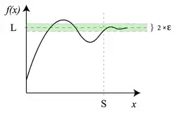
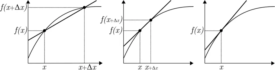
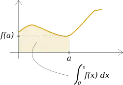
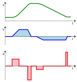


![{\displaystyle =\left[(x+2)\times (x+3)\right]\times \left({\frac {1}{x+3}}\right)}](../_assets_/eb734a37dd21ce173a46342d1cc64c92/00f792cbaa95e7173b24f987832a7ca3cb5134c4.svg)
![{\displaystyle =(x+2)\times \left[(x+3)\times \left({\frac {1}{x+3}}\right)\right]}](../_assets_/eb734a37dd21ce173a46342d1cc64c92/63e733583a409e72d3e6cf410f4aeaa579491bfb.svg)


![{\displaystyle [2,4]}](../_assets_/eb734a37dd21ce173a46342d1cc64c92/e34ad1554b1763ca516be3e0343c4e5b7503a6a0.svg)

![{\displaystyle (2,4]}](../_assets_/eb734a37dd21ce173a46342d1cc64c92/95f52b9b2ea041f44cbbb81e8bd575b236cfaace.svg)


![{\displaystyle [a,b]}](../_assets_/eb734a37dd21ce173a46342d1cc64c92/9c4b788fc5c637e26ee98b45f89a5c08c85f7935.svg)


![{\displaystyle (a,b]}](../_assets_/eb734a37dd21ce173a46342d1cc64c92/6a6969e731af335df071e247ee7fb331cd1a57ae.svg)


![{\displaystyle (-\infty ,a]}](../_assets_/eb734a37dd21ce173a46342d1cc64c92/aeced831f088e701d1985fb783959d2309e0d32a.svg)


![{\displaystyle 2\in [1,3]}](../_assets_/eb734a37dd21ce173a46342d1cc64c92/0a3329d10ef6c978f0960fb9198ed04f74121e52.svg)


![{\displaystyle a^{\frac {m}{n}}={\sqrt[{n}]{a^{m}}}=({\sqrt[{n}]{a}})^{m}}](../_assets_/eb734a37dd21ce173a46342d1cc64c92/c27335eba4c1d0546f4d3617c1700aef479f082f.svg)
![{\displaystyle {\sqrt[{n}]{a}}}](../_assets_/eb734a37dd21ce173a46342d1cc64c92/d7873203eb76042fcd24056c553de8c86054a2df.svg)


![{\displaystyle {\sqrt[{c}]{a^{b}}}}](../_assets_/eb734a37dd21ce173a46342d1cc64c92/d5895c24b750d771f4ef3e0316fc03b4154c2e0f.svg)

![{\displaystyle \left({\frac {1}{8}}\right)^{\frac {1}{2}}={\sqrt[{2}]{\left({\frac {1}{8}}\right)^{1}}}={\sqrt {\frac {1}{8}}}}](../_assets_/eb734a37dd21ce173a46342d1cc64c92/94f5c23d51b8e943f8013a14e79bffef64aeed94.svg)


![{\displaystyle \log _{b}{\sqrt[{c}]{a}}={\frac {\log _{b}a}{c}}}](../_assets_/eb734a37dd21ce173a46342d1cc64c92/7b28fcef6627c1565bccd78fc044f97573b7940d.svg)


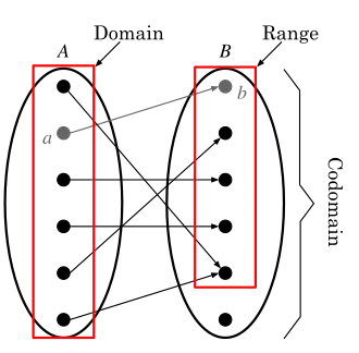


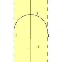


![{\displaystyle x\in [-1,1]}](../_assets_/eb734a37dd21ce173a46342d1cc64c92/1f9d0dda56ce3e01e14570ac9aef0021c6125722.svg)
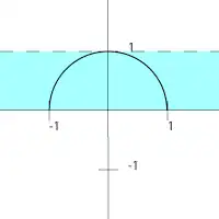
![{\displaystyle f(x)\in [0,1]}](../_assets_/eb734a37dd21ce173a46342d1cc64c92/99f503c443788a9b9f65ff7a48589ce6fd1965d6.svg)
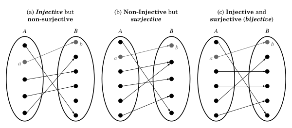


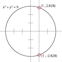


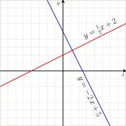


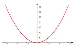


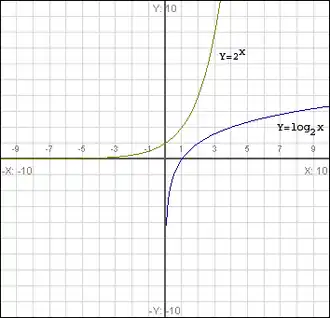


![{\displaystyle x_{1}\in [a,b]}](../_assets_/eb734a37dd21ce173a46342d1cc64c92/0f03ee615e7879f20efa45f3c3c6296c14b53995.svg)
![{\displaystyle x_{2}\in [a,b]}](../_assets_/eb734a37dd21ce173a46342d1cc64c92/e93c068e15bd53700224ed82f922c758216ee03e.svg)


![{\displaystyle x_{1},x_{2}\in [-\infty ,-1]}](../_assets_/eb734a37dd21ce173a46342d1cc64c92/0cf5c7151b951ae1ff019d7e81b7649743e9a8ac.svg)


![{\displaystyle x_{1},x_{2}\in [-1,1]}](../_assets_/eb734a37dd21ce173a46342d1cc64c92/8ed87fe12ce57afdf247fb00036ed2503255e93f.svg)


![{\displaystyle x_{1},x_{2}\in [1,\infty ]}](../_assets_/eb734a37dd21ce173a46342d1cc64c92/740ee44dae32033ccc8b24018acf55e6c11fa60a.svg)


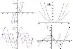


![{\displaystyle \Leftrightarrow x=2[f^{-1}(x)]-7}](../_assets_/eb734a37dd21ce173a46342d1cc64c92/d823629e07ebfdf4e31604db723251807f12fd12.svg)
![{\displaystyle \Leftrightarrow x+7=2[f^{-1}(x)]}](../_assets_/eb734a37dd21ce173a46342d1cc64c92/5ef00069307c01d1d32178da59bf982da21648af.svg)


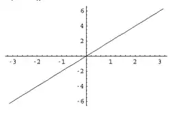


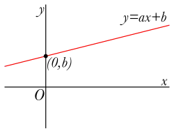


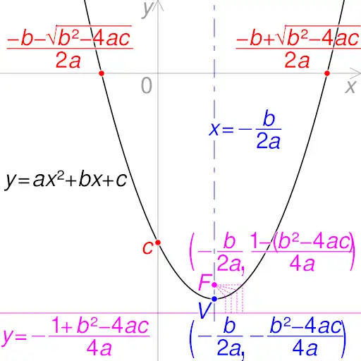


![{\displaystyle [3,4]}](../_assets_/eb734a37dd21ce173a46342d1cc64c92/64d8f09a49d36a9b65d0a754c150774671994b02.svg)


![{\displaystyle {\sqrt[{3}]{\frac {27}{8}}}}](../_assets_/eb734a37dd21ce173a46342d1cc64c92/c81839c276466ff1ed552c297e24958adeda30c7.svg)


![{\displaystyle {\frac {\sqrt {27}}{\sqrt[{3}]{9}}}}](../_assets_/eb734a37dd21ce173a46342d1cc64c92/b940bef569d6d574c586d438a4cc7e69237a9024.svg)


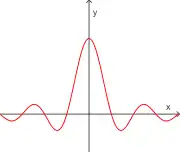


![{\displaystyle \lim _{x\to c}{\Big [}f(x)+g(x){\Big ]}=\lim _{x\to c}f(x)+\lim _{x\to c}g(x)=L+M}](../_assets_/eb734a37dd21ce173a46342d1cc64c92/63558973f7dd0b0f40d8b5ec75c0069be55cbfd5.svg)
![{\displaystyle \lim _{x\to c}{\Big [}f(x)-g(x){\Big ]}=\lim _{x\to c}f(x)-\lim _{x\to c}g(x)=L-M}](../_assets_/eb734a37dd21ce173a46342d1cc64c92/2245bcbbf23e62d18e911d97fb3374f21029d253.svg)
![{\displaystyle \lim _{x\to c}{\Big [}f(x)\cdot g(x){\Big ]}=\lim _{x\to c}f(x)\cdot \lim _{x\to c}g(x)=L\cdot M}](../_assets_/eb734a37dd21ce173a46342d1cc64c92/8bb3a49fa4c6cf42d9198a0a3a589f0d37f801ef.svg)


![{\displaystyle \lim _{x\to 2}{\Big [}4x^{3}+5x+7{\Big ]}}](../_assets_/eb734a37dd21ce173a46342d1cc64c92/b9aa0dd59f814b3b6360f3bf16731fe0ce310506.svg)


![{\displaystyle \lim _{x\to 2}{\Big [}4x^{3}+5x+7{\Big ]}=\lim _{x\to 2}4x^{3}+\lim _{x\to 2}5x+\lim _{x\to 2}7=32+10+7=49}](../_assets_/eb734a37dd21ce173a46342d1cc64c92/89f353a2c991ed44a76cbe15ec92e1a7cef64b59.svg)

![{\displaystyle \lim _{x\to 2}{\Big [}4x^{3}+5x+7{\Big ]}=49}](../_assets_/eb734a37dd21ce173a46342d1cc64c92/353024d0a21d472b9fcc214957ec24ba2bba2071.svg)
![{\displaystyle \lim _{x\to 2}(x-4)(x+10)=\lim _{x\to 2}{\big [}x-4{\big ]}\cdot \lim _{x\to 2}{\big [}x+10{\big ]}=(2-4)(2+10)=-24}](../_assets_/eb734a37dd21ce173a46342d1cc64c92/65c63b2f02d6f5fcce2f8d9f4a03197753b87877.svg)


![{\displaystyle \lim _{x\to 4}{\frac {x^{4}-16x+7}{4x-5}}={\frac {\lim \limits _{x\to 4}{\Big [}x^{4}-16x+7{\Big ]}}{\lim \limits _{x\to 4}{\Big [}4x-5{\Big ]}}}={\frac {\lim \limits _{x\to 4}x^{4}-\lim \limits _{x\to 4}16x+\lim \limits _{x\to 4}7}{\lim \limits _{x\to 4}4x-\lim \limits _{x\to 4}5}}}](../_assets_/eb734a37dd21ce173a46342d1cc64c92/7642ef2f4b9658fcf3b321603072b3855871b00c.svg)


![{\displaystyle \lim _{x\to 0}\left[{\frac {1-\cos(x)}{x}}\right]}](../_assets_/eb734a37dd21ce173a46342d1cc64c92/439aaecbbba70015d6ba2bc0dbbdb28af2a4c879.svg)


![{\displaystyle =\lim _{x\to 0}\left[{\frac {1-\cos(x)}{x}}\cdot {\frac {1}{1}}\right]}](../_assets_/eb734a37dd21ce173a46342d1cc64c92/004dae8cac61686c58224237354804a0103ebd9a.svg)
![{\displaystyle =\lim _{x\to 0}\left[{\frac {1-\cos(x)}{x}}\cdot {\frac {1+\cos(x)}{1+\cos(x)}}\right]}](../_assets_/eb734a37dd21ce173a46342d1cc64c92/b7224657c3fd7b37a16b7a5588b984dda8bc95b3.svg)


![{\displaystyle =\lim _{x\to 0}\left[{\frac {\sin(x)}{x}}\cdot {\frac {\sin(x)}{1+\cos(x)}}\right]}](../_assets_/eb734a37dd21ce173a46342d1cc64c92/d41ba3366a2096441341036c51d162bec854de87.svg)
![{\displaystyle \lim _{x\to 0}\left[{\frac {\sin(x)}{x}}\right]\cdot \lim _{x\to 0}\left[{\frac {\sin(x)}{1+\cos(x)}}\right]}](../_assets_/eb734a37dd21ce173a46342d1cc64c92/01925eba7f3f6d88a6cb8834c53788681d75b7a5.svg)
![{\displaystyle \lim _{x\to 0}\left[{\frac {\sin(x)}{x}}\right]=1}](../_assets_/eb734a37dd21ce173a46342d1cc64c92/160f1b5c8451bba4f762d0423a4ddf0b4c06b44f.svg)
![{\displaystyle \lim _{x\to 0}\left[{\frac {\sin(x)}{1+\cos(x)}}\right]={\frac {\lim \limits _{x\to 0}{\big [}\sin(x){\big ]}}{\lim \limits _{x\to 0}{\big [}1+\cos(x){\big ]}}}={\frac {0}{1+\cos(0)}}=0}](../_assets_/eb734a37dd21ce173a46342d1cc64c92/3162bb4a9f849e9fce9bed16c245dd028f15052a.svg)

![{\displaystyle \lim _{x\to 1}{\bigg [}\sin(x^{2})+4\cos ^{3}(3x-1){\bigg ]}=\sin(1^{2})+4\cos ^{3}(3\cdot 1-1)=\sin 1+4\cos ^{3}2}](../_assets_/eb734a37dd21ce173a46342d1cc64c92/57ef4597d5d1294ea634e4d530898e083ed19734.svg)


![{\displaystyle [-2,2]}](../_assets_/eb734a37dd21ce173a46342d1cc64c92/f94b820404eca2a458cb2c7d8c24be85fffccf90.svg)

.svg.png)

![{\displaystyle (0,{\tfrac {1}{\pi }}]}](../_assets_/eb734a37dd21ce173a46342d1cc64c92/f41cc2319c9c4acc7cd957eb6a02fc6070fa869a.svg)


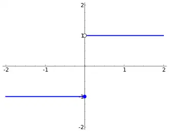


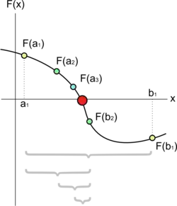
![{\displaystyle [a_{1},b_{1}]}](../_assets_/eb734a37dd21ce173a46342d1cc64c92/90b50cd52227fb045ffb69b5802b79b7b539e8d2.svg)


![{\displaystyle [-1,1]}](../_assets_/eb734a37dd21ce173a46342d1cc64c92/51e3b7f14a6f70e614728c583409a0b9a8b9de01.svg)
![{\displaystyle (0,1]}](../_assets_/eb734a37dd21ce173a46342d1cc64c92/7e70f9c241f9faa8e9fdda2e8b238e288807d7a4.svg)


![{\displaystyle \lim _{x\to a}{\big [}f(x)+g(x){\big ]}}](../_assets_/eb734a37dd21ce173a46342d1cc64c92/38060b7158f65e3a3b93578e271e872b054a8682.svg)


![{\displaystyle \lim _{x\to c}{\Big [}f(x)+g(x){\Big ]}}](../_assets_/eb734a37dd21ce173a46342d1cc64c92/31c6d4f3cc8728d7e72b0f426657955d0cb1b383.svg)


![{\displaystyle \lim _{x\to c}{\Big [}f(x)-g(x){\Big ]}=\lim _{x\to c}{\Big [}f(x)+h(x){\Big ]}=L-M}](../_assets_/eb734a37dd21ce173a46342d1cc64c92/8928557687932b07789eb9ee3cb1b4b4125b8065.svg)


![{\displaystyle \lim _{x\to 2}{\Big [}4x^{2}-3x-1{\Big ]}}](../_assets_/eb734a37dd21ce173a46342d1cc64c92/b9090ef0539e55c8c495638167af1902f6c0371e.svg)
![{\displaystyle \lim _{x\to 5}{\Big [}x^{2}{\Big ]}}](../_assets_/eb734a37dd21ce173a46342d1cc64c92/ddef2e7715fea4bcb0a1fdacbcc14b5049a50a46.svg)
![{\displaystyle \lim _{x\to {\frac {\pi }{4}}}{\Big [}\cos ^{2}(x){\Big ]}}](../_assets_/eb734a37dd21ce173a46342d1cc64c92/b2b628dde4a64c213ceea9a932bba29f50ebe270.svg)
![{\displaystyle \lim _{x\to 1}{\Big [}5e^{x-1}-5{\Big ]}}](../_assets_/eb734a37dd21ce173a46342d1cc64c92/1fbd3c44c22819b3d1cfe0b427d665f4742f96bc.svg)

![{\displaystyle \lim _{x\to 7^{-}}{\Big [}|x^{2}+x|-x{\Big ]}}](../_assets_/eb734a37dd21ce173a46342d1cc64c92/107d70cb67026562a0c3ed9db454d47178947b2b.svg)


![{\displaystyle \lim _{x\to 1}\left[x^{2}+5x-{\frac {1}{2-x}}\right]}](../_assets_/eb734a37dd21ce173a46342d1cc64c92/00ff82956e4812c90be92af6b92fe043d09fec3c.svg)


![{\displaystyle \lim _{x\to -\infty }{\Big [}3x^{2}-2x+1{\Big ]}}](../_assets_/eb734a37dd21ce173a46342d1cc64c92/5a9cfb494972698a81cd5a92200191100d2baff1.svg)


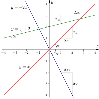


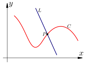
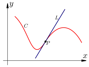
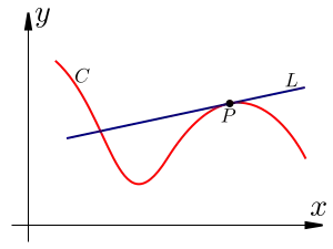
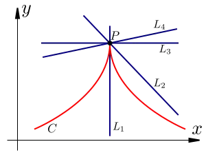
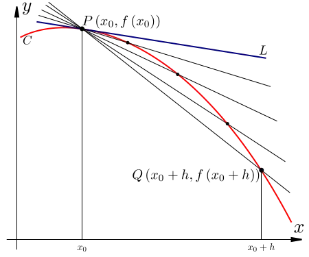


![{\displaystyle \lim _{h\to 0}\left[{\frac {f(x_{0}+h)-f(x_{0})}{h}}\right]}](../_assets_/eb734a37dd21ce173a46342d1cc64c92/4d4bd8965a03018d783a87573829f2113ec86fb4.svg)


![{\displaystyle D_{x}[f(x)]}](../_assets_/eb734a37dd21ce173a46342d1cc64c92/d0bc0c64c0455d3e24668b95c4790e57806572f3.svg)

![{\displaystyle {\frac {d}{dx}}{\big [}y{\big ]}}](../_assets_/eb734a37dd21ce173a46342d1cc64c92/d7a51a0607b2d4e9448055729d46246c4c9dc429.svg)


![{\displaystyle {\frac {d}{dx}}[c]=0}](../_assets_/eb734a37dd21ce173a46342d1cc64c92/834381b512bc1d1fc47c2d26ce38ae71daaa1053.svg)


![{\displaystyle {\frac {d}{dx}}[c]=\lim _{\Delta x\to 0}{\frac {c-c}{\Delta x}}=\lim _{\Delta x\to 0}{\frac {0}{\Delta x}}}](../_assets_/eb734a37dd21ce173a46342d1cc64c92/a6429024c32c4dcbfab9e4f461bbf7c250e51f94.svg)


![{\displaystyle {\frac {d}{dx}}[3]=0}](../_assets_/eb734a37dd21ce173a46342d1cc64c92/4971c461d4d1899584259a8cc861f594a720bfc6.svg)
![{\displaystyle {\frac {d}{dx}}[z]=0}](../_assets_/eb734a37dd21ce173a46342d1cc64c92/43ee2f6002376e773eb77e8027a8b9969e6fa186.svg)

![{\displaystyle {\frac {d}{dx}}[mx+c]=m}](../_assets_/eb734a37dd21ce173a46342d1cc64c92/a2233b08b6e33432899e0a6e4b5f10c04fa80180.svg)


![{\displaystyle {\frac {d}{dx}}{\big [}c\cdot f(x){\big ]}=c\cdot {\frac {d}{dx}}{\big [}f(x){\big ]}}](../_assets_/eb734a37dd21ce173a46342d1cc64c92/620f42e9b7e02ab5849561b877d00e9f3991cc9c.svg)
![{\displaystyle {\frac {d}{dx}}{\big [}x^{2}{\big ]}=2x}](../_assets_/eb734a37dd21ce173a46342d1cc64c92/a3f98d70aed6c89c1d7a7aa3afb8fa65cc1370d2.svg)

![{\displaystyle {\frac {d}{dx}}{\big [}3x^{2}{\big ]}}](../_assets_/eb734a37dd21ce173a46342d1cc64c92/2bec61ad4893c0105e6ca724cc569f579acef837.svg)
![{\displaystyle =3{\frac {d}{dx}}{\big [}x^{2}{\big ]}}](../_assets_/eb734a37dd21ce173a46342d1cc64c92/269595874a5ae15117c9b2ac88adc77f294b1f02.svg)

![{\displaystyle {\frac {d}{dx}}{\big [}f(x)\pm g(x){\big ]}={\frac {d}{dx}}{\big [}f(x){\big ]}\pm {\frac {d}{dx}}{\big [}g(x){\big ]}}](../_assets_/eb734a37dd21ce173a46342d1cc64c92/7aac5a3d2b8cb3ec27547f593f51f3623d6649f8.svg)
![{\displaystyle \lim _{\Delta x\to 0}\left[{\frac {{\big [}f(x+\Delta x)\pm g(x+\Delta x){\big ]}-{\big [}f(x)\pm g(x){\big ]}}{\Delta x}}\right]}](../_assets_/eb734a37dd21ce173a46342d1cc64c92/b4ed1e8360a288ade75ddcb507e376dd9cee55ec.svg)
![{\displaystyle =\lim _{\Delta x\to 0}\left[{\frac {{\big [}f(x+\Delta x)-f(x){\big ]}\pm {\big [}g(x+\Delta x)-g(x){\big ]}}{\Delta x}}\right]}](../_assets_/eb734a37dd21ce173a46342d1cc64c92/0ee0f6b5bb2a556f430421f7480eaea10469c133.svg)
![{\displaystyle =\lim _{\Delta x\to 0}\left[{\frac {f(x+\Delta x)-f(x)}{\Delta x}}\right]\pm \lim _{\Delta x\to 0}\left[{\frac {g(x+\Delta x)-g(x)}{\Delta x}}\right]}](../_assets_/eb734a37dd21ce173a46342d1cc64c92/406f621d8790d9044a333148e0bb949e1af537ee.svg)
![{\displaystyle {\frac {d}{dx}}\left[f(x)\right]\pm {\frac {d}{dx}}\left[g(x)\right]}](../_assets_/eb734a37dd21ce173a46342d1cc64c92/ef506c07a97f260c7649fd622782c878eaaff692.svg)

![{\displaystyle {\frac {d}{dx}}{\big [}3x^{2}+5x{\big ]}}](../_assets_/eb734a37dd21ce173a46342d1cc64c92/93c9a04e8e8a83377a5f87ff165c4e0081b881ca.svg)
![{\displaystyle ={\frac {d}{dx}}{\big [}3x^{2}+5x{\big ]}}](../_assets_/eb734a37dd21ce173a46342d1cc64c92/c95485942f79fba6dafa06b3994d360a65a3b747.svg)
![{\displaystyle ={\frac {d}{dx}}{\big [}3x^{2}{\big ]}+{\frac {d}{dx}}{\big [}5x{\big ]}}](../_assets_/eb734a37dd21ce173a46342d1cc64c92/d5fe7f0830a02ef2c17ba626724dc42b8f624708.svg)
![{\displaystyle =6x+{\frac {d}{dx}}{\big [}5x{\big ]}}](../_assets_/eb734a37dd21ce173a46342d1cc64c92/40d69fd1b86b44bb1d43a9ec7fe819172ec0d523.svg)

![{\displaystyle {\frac {d}{dx}}{\big [}x^{n}{\big ]}=nx^{n-1}}](../_assets_/eb734a37dd21ce173a46342d1cc64c92/5ea2db0416ac0c9b3364fb54cc2e99d9342249df.svg)


![{\displaystyle {\frac {d}{dx}}{\big [}{\sqrt {x}}{\big ]}}](../_assets_/eb734a37dd21ce173a46342d1cc64c92/7569884584a27c56af7a5333731d7a2d332e63ce.svg)
![{\displaystyle ={\frac {d}{dx}}{\big [}x^{\frac {1}{2}}{\big ]}}](../_assets_/eb734a37dd21ce173a46342d1cc64c92/d7e66c17740cb48dc20d868a786193340fa4ba35.svg)


![{\displaystyle {\frac {d}{dx}}{\big [}6x^{5}+3x^{2}+3x+1{\big ]}}](../_assets_/eb734a37dd21ce173a46342d1cc64c92/68013f0aa462e583c6cab1228a3f2cd9f81c9645.svg)
![{\displaystyle {\frac {d}{dx}}{\big [}6x^{5}{\big ]}+{\frac {d}{dx}}{\big [}3x^{2}{\big ]}+{\frac {d}{dx}}{\big [}3x{\big ]}+{\frac {d}{dx}}[1]}](../_assets_/eb734a37dd21ce173a46342d1cc64c92/0adbd7509b1658e1b79408313dc3e439753abb10.svg)
![{\displaystyle {\frac {d}{dx}}{\big [}6x^{5}{\big ]}+{\frac {d}{dx}}{\big [}3x^{2}{\big ]}+3+0}](../_assets_/eb734a37dd21ce173a46342d1cc64c92/399baa9d1f7a4b71032acd1e2731dab17809b790.svg)
![{\displaystyle 6{\frac {d}{dx}}{\big [}x^{5}{\big ]}+3{\frac {d}{dx}}{\big [}x^{2}{\big ]}+3}](../_assets_/eb734a37dd21ce173a46342d1cc64c92/ada9b3269f5fd71e399f6280c6881d85809f461a.svg)


![{\displaystyle {\frac {d}{dx}}{\Big [}f(x)\cdot g(x){\Big ]}=f'(x)\cdot g(x)+f(x)\cdot g'(x)}](../_assets_/eb734a37dd21ce173a46342d1cc64c92/fa57a3aa4e93fe8a5a8dfd15d88761d0d331be18.svg)


![{\displaystyle v(t)={\frac {d}{dt}}{\Big [}4t^{3}\tan(t)\sec(t){\Big ]}=\tan(t)\sec(t)\cdot {\frac {d}{dt}}[4t^{3}]+4t^{3}\sec(t)\cdot {\frac {d}{dt}}[\tan(t)]+4t^{3}\tan(t)\cdot {\frac {d}{dt}}[\sec(t)]}](../_assets_/eb734a37dd21ce173a46342d1cc64c92/ece0bc18f9189f0b36823b14c86a59d209362d08.svg)


![{\displaystyle {\frac {d}{dx}}{\Big [}f(x)\cdot g(x){\Big ]}=\lim _{h\to 0}{\frac {f(x+h)\cdot g(x+h)-f(x)\cdot g(x)}{h}}}](../_assets_/eb734a37dd21ce173a46342d1cc64c92/52de234ae8c19cd0fbd5f68f4358d72c7e9940df.svg)
![{\displaystyle {\frac {d}{dx}}{\Big [}f(x)\cdot g(x){\Big ]}=\lim _{h\to 0}{\frac {f(x+h)\cdot g(x+h)-{\color {blue}f(x+h)\cdot g(x)+f(x+h)\cdot g(x)}-f(x)\cdot g(x)}{h}}}](../_assets_/eb734a37dd21ce173a46342d1cc64c92/2bda4b55f097600c6ecd29d6ea86ed0b174bb66d.svg)
![{\displaystyle {\frac {d}{dx}}{\Big [}f(x)\cdot g(x){\Big ]}=\lim _{h\to 0}\left[{\frac {f(x+h)\cdot g(x+h)-f(x+h)\cdot g(x)}{h}}+{\frac {f(x+h)\cdot g(x)-f(x)\cdot g(x)}{h}}\right]}](../_assets_/eb734a37dd21ce173a46342d1cc64c92/b3c8778519c923a41496315260334543ce505ac3.svg)
![{\displaystyle {\begin{aligned}{\frac {d}{dx}}{\Big [}f(x)\cdot g(x){\Big ]}&=\lim _{h\to 0}\left[f(x+h)\cdot {\frac {g(x+h)-g(x)}{h}}+g(x)\cdot {\frac {f(x+h)-f(x)}{h}}\right]\\&=\lim _{h\to 0}\left[f(x+h)\cdot {\frac {g(x+h)-g(x)}{h}}\right]+\lim _{h\to 0}\left[g(x)\cdot {\frac {f(x+h)-f(x)}{h}}\right]\\&=\lim _{h\to 0}f(x+h)\cdot \lim _{h\to 0}{\frac {g(x+h)-g(x)}{h}}+\lim _{h\to 0}g(x)\cdot \lim _{h\to 0}{\frac {f(x+h)-f(x)}{h}}\end{aligned}}}](../_assets_/eb734a37dd21ce173a46342d1cc64c92/dee68cf3d65c2562d300e7762ab1549aa7c98e25.svg)
![{\displaystyle {\frac {d}{dx}}{\Big [}f(x)\cdot g(x){\Big ]}=f(x)\cdot g'(x)+f'(x)\cdot g(x)}](../_assets_/eb734a37dd21ce173a46342d1cc64c92/3722599709398f767756759b3099007ae28c191a.svg)
![{\displaystyle {\frac {d}{dx}}[f\cdot g\cdot h]=f(x)g(x)h'(x)+f(x)g'(x)h(x)+f'(x)g(x)h(x)}](../_assets_/eb734a37dd21ce173a46342d1cc64c92/99735dd3a693a9ec554c7a2d964ee20dc7634471.svg)


![{\displaystyle {\begin{aligned}{\frac {d}{dx}}\left[{\frac {f(x)}{g(x)}}\right]&=\lim _{h\to 0}{\dfrac {{\dfrac {f(x+h)}{g(x+h)}}-{\dfrac {f(x)}{g(x)}}}{h}}\\\\&=\lim _{h\to 0}{\frac {f(x+h)\cdot g(x)-f(x)\cdot g(x+h)}{h\cdot g(x)\cdot g(x+h)}}\\\\&=\lim _{h\to 0}{\frac {f(x+h)\cdot g(x)-{\color {blue}f(x)\cdot g(x)+f(x)\cdot g(x)}-f(x)\cdot g(x+h)}{h\cdot g(x)\cdot g(x+h)}}\\\\&=\lim _{h\to 0}{\dfrac {g(x)\cdot {\dfrac {f(x+h)-f(x)}{h}}-f(x)\cdot {\dfrac {g(x+h)-g(x)}{h}}}{g(x)\cdot g(x+h)}}\\\\&={\dfrac {\lim \limits _{h\to 0}\left[g(x)\cdot {\dfrac {f(x+h)-f(x)}{h}}-f(x)\cdot {\dfrac {g(x+h)-g(x)}{h}}\right]}{\lim \limits _{h\to 0}{\Big [}g(x)\cdot g(x+h){\Big ]}}}\\\\&={\dfrac {\lim \limits _{h\to 0}\left[g(x)\cdot {\dfrac {f(x+h)-f(x)}{h}}\right]-\lim \limits _{h\to 0}\left[f(x)\cdot {\dfrac {g(x+h)-g(x)}{h}}\right]}{\lim \limits _{h\to 0}{\Big [}g(x)\cdot g(x+h){\Big ]}}}\\\\&={\dfrac {\lim \limits _{h\to 0}g(x)\cdot \lim \limits _{h\to 0}{\dfrac {f(x+h)-f(x)}{h}}-\lim \limits _{h\to 0}f(x)\cdot \lim \limits _{h\to 0}{\dfrac {g(x+h)-g(x)}{h}}}{\lim \limits _{h\to 0}g(x)\cdot \lim \limits _{h\to 0}g(x+h)}}\\\\&={\frac {f'(x)g(x)-f(x)g'(x)}{g(x)^{2}}}\end{aligned}}}](../_assets_/eb734a37dd21ce173a46342d1cc64c92/64a5758e93c0b14096dfc5b1935d7fbf8f0917c9.svg)
![{\displaystyle {\frac {d}{dx}}\left[{\frac {f(x)}{g(x)}}\right]={\frac {g(x)f'(x)-f(x)g'(x)}{g(x)^{2}}}}](../_assets_/eb734a37dd21ce173a46342d1cc64c92/bb4eb3cc163187d7c13cd091f727db380a0770ac.svg)

![{\displaystyle {\begin{aligned}{\frac {d}{dx}}\left[{\frac {4x-2}{x^{2}+1}}\right]&={\frac {(4)(x^{2}+1)-(2x)(4x-2)}{(x^{2}+1)^{2}}}\\&={\frac {(4x^{2}+4)-(8x^{2}-4x)}{(x^{2}+1)^{2}}}\\&={\frac {-4x^{2}+4x+4}{(x^{2}+1)^{2}}}\end{aligned}}}](../_assets_/eb734a37dd21ce173a46342d1cc64c92/80429e152a529cb7131b4a67df46fbc7bc32db8e.svg)


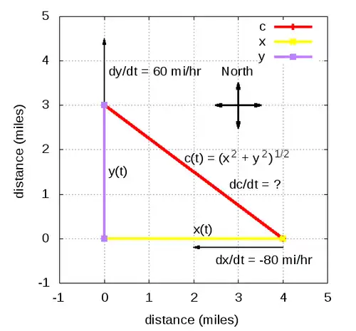


![{\displaystyle ={\frac {(x^{2}+y^{2})^{-{\frac {1}{2}}}}{2}}\left[{\frac {d}{dt}}(x^{2})+{\frac {d}{dt}}(y^{2})\right]}](../_assets_/eb734a37dd21ce173a46342d1cc64c92/a9b656c37ba8c39165514d9c4f0aa65607823dec.svg)
![{\displaystyle ={\frac {(x^{2}+y^{2})^{-{\frac {1}{2}}}}{2}}\left[2x\cdot {\frac {dx}{dt}}+2y\cdot {\frac {dy}{dt}}\right]}](../_assets_/eb734a37dd21ce173a46342d1cc64c92/bcb61fdaf2803d1535e1cc73516ecb68202d807b.svg)


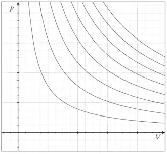


![{\displaystyle {\frac {d^{2}}{dx^{2}}}[f(x)]}](../_assets_/eb734a37dd21ce173a46342d1cc64c92/ad0399ac042750a6f46e6e7e6c96ae6c72338adf.svg)
![{\displaystyle {\frac {d^{3}}{dx^{3}}}[f(x)]}](../_assets_/eb734a37dd21ce173a46342d1cc64c92/035520219482358aa12ce353b11784c9927acf01.svg)
![{\displaystyle {\frac {d^{4}}{dx^{4}}}[f(x)]}](../_assets_/eb734a37dd21ce173a46342d1cc64c92/1995a4c7ceafe37c7696a11e4d507a809a5966a8.svg)
![{\displaystyle {\frac {d^{n}}{dx^{n}}}[f(x)]}](../_assets_/eb734a37dd21ce173a46342d1cc64c92/8238d8b3d21d91a36e57b7816790f394c52fa8db.svg)


![{\displaystyle {\frac {dy}{dx}}={\frac {d}{dx}}[f(x)]=f'(x)}](../_assets_/eb734a37dd21ce173a46342d1cc64c92/5326dab9b69c29a51068061c1f34ceabf1ac8a03.svg)


![{\displaystyle {\frac {d}{dx}}{\bigl [}f{\bigl (}x,y(x){\bigr )}{\bigr ]}={\frac {d}{dx}}{\big [}g{\bigl (}x,y(x){\bigr )}{\big ]}}](../_assets_/eb734a37dd21ce173a46342d1cc64c92/6016d795e7556324ef64947c8f84f10be41ffea6.svg)
![{\displaystyle {\frac {d}{dx}}(y^{3})={\frac {d}{dy}}[y^{3}]\cdot {\frac {dy}{dx}}=3y^{2}\cdot y'}](../_assets_/eb734a37dd21ce173a46342d1cc64c92/f5d3b59fad82ccce72ecf27b8e1675128c39404d.svg)

![{\displaystyle {\frac {d}{dx}}{\bigl [}f{\bigl (}g(x){\bigr )}{\bigr ]}=f'{\bigl (}g(x){\bigr )}\cdot g'(x)}](../_assets_/eb734a37dd21ce173a46342d1cc64c92/e596118af0cab829b12dec0a6f0ee05d4f242694.svg)


![{\displaystyle {\frac {d}{dx}}{\bigl [}f{\bigl (}y(x){\bigr )}{\bigr ]}=f'{\bigl (}y(x){\bigr )}\cdot y'(x)=2y(x)y'(x)}](../_assets_/eb734a37dd21ce173a46342d1cc64c92/57a24127aed120ea4e263f431119c0502cf494e4.svg)


![{\displaystyle {\frac {d}{dx}}[x^{2}+y^{2}]={\frac {d}{dx}}[1]}](../_assets_/eb734a37dd21ce173a46342d1cc64c92/00d1e61ce2b704b39884bf0912548093b9241785.svg)
![{\displaystyle {\frac {d}{dx}}[x^{2}]+{\frac {d}{dx}}[y^{2}]=0}](../_assets_/eb734a37dd21ce173a46342d1cc64c92/312afa8f5fb0007e43ed0d3a892552c4a7b9c56d.svg)


![{\displaystyle {\frac {d}{dx}}[xy]={\frac {d}{dx}}[1]}](../_assets_/eb734a37dd21ce173a46342d1cc64c92/b616e67fbda614eaacc9c29cbcbe0abbbe377a63.svg)


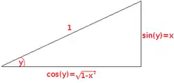


![{\displaystyle {\frac {d}{dx}}[\log _{a}(a^{x})]={\frac {d}{dx}}[x]\implies {\frac {1}{\ln(a)a^{x}}}{\frac {d}{dx}}[a^{x}]=1}](../_assets_/eb734a37dd21ce173a46342d1cc64c92/c80755cd30a9894127445a752fb6854dbf92b3c8.svg)
![{\displaystyle {\frac {d}{dx}}[a^{x}]=a^{x}\ln(a)}](../_assets_/eb734a37dd21ce173a46342d1cc64c92/f91dcc2587e0b8b3bbdc7449f09ae0e3e0b13a6f.svg)


![{\displaystyle {\frac {d}{dx}}[e^{x}]=e^{x}}](../_assets_/eb734a37dd21ce173a46342d1cc64c92/783a58bf19ce36ca7781d7d31d78161a55406bff.svg)


![{\displaystyle x\in [a,b]}](../_assets_/eb734a37dd21ce173a46342d1cc64c92/026357b404ee584c475579fb2302a4e9881b8cce.svg)


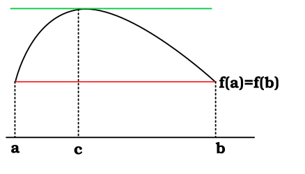


![{\displaystyle [0,\pi ]}](../_assets_/eb734a37dd21ce173a46342d1cc64c92/3e2a912eda6ef1afe46a81b518fe9da64a832751.svg)


![{\displaystyle {\frac {d}{dx}}[c\cdot f(x)]=c\cdot {\frac {d}{dx}}[f(x)]}](../_assets_/eb734a37dd21ce173a46342d1cc64c92/e100ac3ba73695d9c36ad8ada81efba4c2a01129.svg)

![{\displaystyle f(x)=3{\sqrt[{3}]{x}}\,}](../_assets_/eb734a37dd21ce173a46342d1cc64c92/c7b861dfb68b951e23d614557d2cb071669b0851.svg)


![{\displaystyle f(x)={\frac {3}{x^{4}}}-{\sqrt[{4}]{x}}+x}](../_assets_/eb734a37dd21ce173a46342d1cc64c92/ff2d5e5287d1e1f9e9a3f66fe3d81364fbed337c.svg)

![{\displaystyle f(x)={\frac {1}{\sqrt[{3}]{x}}}+{\sqrt {x}}}](../_assets_/eb734a37dd21ce173a46342d1cc64c92/aa56b0f9f1e3f9dbd84b8e241f26eec58e0f966e.svg)


![{\displaystyle {\frac {d}{dx}}[(x^{3}+5)^{10}]}](../_assets_/eb734a37dd21ce173a46342d1cc64c92/322d22bf641e5d6a35d63be10b39c7353404dfcd.svg)
![{\displaystyle {\frac {d}{dx}}[x^{3}+3x]}](../_assets_/eb734a37dd21ce173a46342d1cc64c92/052c718ffadbb9cb4954b7dd5791f055ff1ce77c.svg)
![{\displaystyle {\frac {d}{dx}}[(x+4)(x+2)(x-3)]}](../_assets_/eb734a37dd21ce173a46342d1cc64c92/160ae1c70a96f198eb4c1fd16d0ed2940ce4acfb.svg)
![{\displaystyle {\frac {d}{dx}}[{\frac {x+1}{3x^{2}}}]}](../_assets_/eb734a37dd21ce173a46342d1cc64c92/9320f75bc1f03266f545ee487bd178d212956699.svg)
![{\displaystyle {\frac {d}{dx}}[3x^{3}]}](../_assets_/eb734a37dd21ce173a46342d1cc64c92/d330c0494fcf0513cd524464634f6360c2ed4c23.svg)
![{\displaystyle {\frac {d}{dx}}[x^{4}\sin(x)]}](../_assets_/eb734a37dd21ce173a46342d1cc64c92/c54697e3e6e8b7be626f8ad40a67ef061ab14bde.svg)
![{\displaystyle {\frac {d}{dx}}[2^{x}]}](../_assets_/eb734a37dd21ce173a46342d1cc64c92/70c4dd6b628068248913d496b20327629fc271d2.svg)
![{\displaystyle {\frac {d}{dx}}[e^{x^{2}}]}](../_assets_/eb734a37dd21ce173a46342d1cc64c92/70feadeaf0a4d91cf66a795d8d2f169e942ec523.svg)
![{\displaystyle {\frac {d}{dx}}[e^{2^{x}}]}](../_assets_/eb734a37dd21ce173a46342d1cc64c92/ea1c7dffc918e0d7462c5f97f9a145db84a16597.svg)


![{\displaystyle y=x({\sqrt[{4}]{1-x^{3}}})}](../_assets_/eb734a37dd21ce173a46342d1cc64c92/24d04c97ee04319439a96db44e9efa9e702123a0.svg)


![{\displaystyle [x,a]}](../_assets_/eb734a37dd21ce173a46342d1cc64c92/fd914a696a64f589f9d3d6d295a62aaa94f8045f.svg)
![{\displaystyle [a,x]}](../_assets_/eb734a37dd21ce173a46342d1cc64c92/692f0edd0d40232c8a69ed5de7b142e1e343eff7.svg)


![{\displaystyle \ln(k)=\lim _{x\to \infty }{\frac {\ln \left(1+{\frac {1}{x}}\right)}{\frac {1}{x}}}=\lim _{x\to \infty }{\frac {{\frac {d}{dx}}\left[\ln \left(1+{\frac {1}{x}}\right)\right]}{{\frac {d}{dx}}\left({\frac {1}{x}}\right)}}=\lim _{x\to \infty }{\frac {x}{x+1}}}](../_assets_/eb734a37dd21ce173a46342d1cc64c92/973bf7b09797ca31a0696ae39d48fe73325e8686.svg)


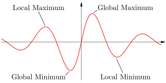

.svg.png)

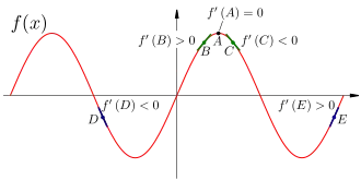


![{\displaystyle [-3,3]}](../_assets_/eb734a37dd21ce173a46342d1cc64c92/3a869f6f7ff84a95f888c6b8705e2465ba21960e.svg)


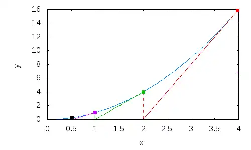


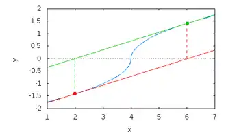


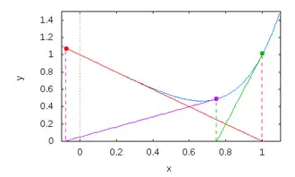


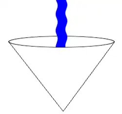


![{\displaystyle {\begin{aligned}V&={\frac {1}{2}}\left[50{\sqrt {\frac {50}{3}}}-\left({\sqrt {\frac {50}{3}}}\right)^{3}\right]\\&=68.04138174...\end{aligned}}}](../_assets_/eb734a37dd21ce173a46342d1cc64c92/1016de1bd948d063b0301102ac8f1d32e5db2c84.svg)

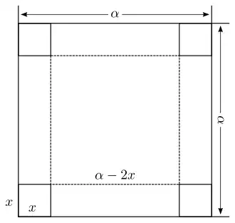


![{\displaystyle \Leftrightarrow r={\sqrt[{3}]{\frac {512}{\pi }}}={\frac {8}{\sqrt[{3}]{\pi }}}\approx 5.4623}](../_assets_/eb734a37dd21ce173a46342d1cc64c92/6e42754b752fade90afad51c224f9689804ee180.svg)


![{\displaystyle r\in \left(0,\,{\frac {8}{\sqrt[{3}]{\pi }}}\right)}](../_assets_/eb734a37dd21ce173a46342d1cc64c92/96915a7d682f5b524441ceb9e088d8ed2fa9b0c8.svg)
![{\displaystyle r\in \left({\frac {8}{\sqrt[{3}]{\pi }}},\,\infty \right)}](../_assets_/eb734a37dd21ce173a46342d1cc64c92/1920a8a9fc78db9999a594921610687e3e17f1d9.svg)


![{\displaystyle r={\frac {8}{\sqrt[{3}]{\pi }}}}](../_assets_/eb734a37dd21ce173a46342d1cc64c92/0752408a203daa5d896bbc99fc8240ab9e9130c6.svg)


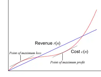


![{\displaystyle p'(n)={\frac {d}{dn}}[8.1n]-{\frac {d}{dn}}\left[n^{3}-7n^{2}+18n\right]=-3n^{2}+14n-9.9}](../_assets_/eb734a37dd21ce173a46342d1cc64c92/d41290e939ddf7f9c86a7f1a4dd9b058b51dd1b7.svg)


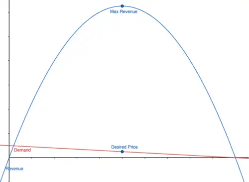


![{\displaystyle {\frac {d}{dq}}\left[R(q)\right]={\frac {d}{dq}}\left[-{\frac {1}{5}}q^{2}+10q\right]}](../_assets_/eb734a37dd21ce173a46342d1cc64c92/96c11ed278243ba6039e38b9b598b58f7a9c5eb1.svg)
![{\displaystyle {\begin{aligned}R'(q)&={\frac {d}{dq}}\left[-{\frac {1}{5}}q^{2}\right]+{\frac {d}{dq}}\left[10q\right]\\&=-{\frac {1}{5}}{\frac {d}{dq}}\left[q^{2}\right]+10{\frac {d}{dq}}\left[q\right]\\&=-{\frac {1}{5}}\left[2q\right]+10\left[1\right]\\&=-{\frac {2}{5}}q+10\end{aligned}}}](../_assets_/eb734a37dd21ce173a46342d1cc64c92/4ba47b1df2588ee473e4585428f9abfa94b26e71.svg)


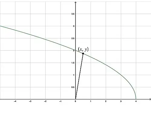


![{\displaystyle \Rightarrow {\frac {d}{dx}}\left[D(x)\right]={\frac {d}{dx}}\left({\sqrt {x^{2}-x+4}}\right)}](../_assets_/eb734a37dd21ce173a46342d1cc64c92/efa97ac067e0b0ee20efd1cd3d5d89c650c248f4.svg)
![{\displaystyle {\begin{aligned}\Rightarrow D'(x)&={\frac {d}{dx}}\left({\sqrt {x^{2}-x+4}}\right)&\left({\text{Recall the chain rule: }}{\frac {d}{dx}}\left[f\left(g(x)\right)\right]={\frac {df}{dg}}\cdot {\frac {dg}{dx}}\right)\\&={\frac {d}{dx}}\left(x^{2}-x+4\right)\cdot {\frac {df}{dg}}\left({\sqrt {x^{2}-x+4}}\right)\\&=\left(2x-1\right)\cdot {\frac {1}{2{\sqrt {x^{2}-x+4}}}}\\&={\frac {2x-1}{2{\sqrt {x^{2}-x+4}}}}\end{aligned}}}](../_assets_/eb734a37dd21ce173a46342d1cc64c92/90809dbc1c9072ae0d6765f5fcb83e302a884d8f.svg)


![{\displaystyle \left[D(x)\right]^{2}=x^{2}-x+4}](../_assets_/eb734a37dd21ce173a46342d1cc64c92/9281d15377d26c437c929bd60828d32149628d30.svg)
![{\displaystyle {\frac {d}{dx}}\left[\left(D(x)\right)^{2}\right]={\frac {d}{dx}}\left(x^{2}-x+4\right)}](../_assets_/eb734a37dd21ce173a46342d1cc64c92/b120f7dd809b08541f60d50eb4084fa86e84a5c0.svg)


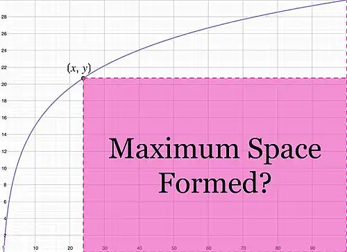


![{\displaystyle \Rightarrow {\frac {d}{dx}}\left[A(x)\right]={\frac {d}{dx}}\left[15(100-x)\log(x)\right]}](../_assets_/eb734a37dd21ce173a46342d1cc64c92/683a6bd7b28c38b48c913df1248b49525539348f.svg)
![{\displaystyle {\begin{aligned}\Rightarrow A'(x)&=15{\frac {d}{dx}}\left((100-x)\log(x)\right)&\left({\text{Recall the product rule: }}{\frac {d}{dx}}\left[f(x)\cdot g(x)\right]=f\cdot {\frac {dg}{dx}}+g\cdot {\frac {df}{dx}}\right)\\&=15\left[(100-x)\cdot {\frac {d}{dx}}\left(\log(x)\right)+\log(x)\cdot {\frac {d}{dx}}\left(100-x\right)\right]\\&=15\left[{\frac {100-x}{x\ln(10)}}-\log(x)\right]\\&=15\left[{\frac {100-x}{x\ln(10)}}-{\frac {\ln(x)}{\ln(10)}}\right]&\left({\text{Multiply by }}{\frac {x}{x}}{\text{ to the right fraction.}}\right)\\&=15\left[{\frac {100-x}{x\ln(10)}}-{\frac {x\ln(x)}{x\ln(10)}}\right]\\&=15\left[{\frac {100-x-x\ln(x)}{x\ln(10)}}\right]=0\\\end{aligned}}}](../_assets_/eb734a37dd21ce173a46342d1cc64c92/202126144026256e023e854186c9039cbf379767.svg)


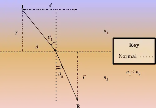


![{\displaystyle {\frac {d}{d\Lambda }}\left[T(\Lambda )\right]={\frac {d}{d\Lambda }}\left({\frac {\sqrt {\Lambda ^{2}+\Upsilon ^{2}}}{v_{1}}}+{\frac {\sqrt {(d-\Lambda )^{2}+\Gamma ^{2}}}{v_{2}}}\right)}](../_assets_/eb734a37dd21ce173a46342d1cc64c92/d3c799390bf0c8dca50585f1929a45c9867b9e1b.svg)


.svg.png)


![{\displaystyle f(x)={\sqrt[{3}]{(x-1)^{2}}}}](../_assets_/eb734a37dd21ce173a46342d1cc64c92/f4371183376851214640d374c3917162fc7ee8ac.svg)


![{\displaystyle [0,3]}](../_assets_/eb734a37dd21ce173a46342d1cc64c92/d5c9e70f7d437509d4ebedb0eaf7ada946e91a79.svg)

![{\displaystyle [-{\tfrac {1}{2}},2]}](../_assets_/eb734a37dd21ce173a46342d1cc64c92/ad45dba0e31544218eea18079f13e69dc265793f.svg)


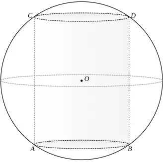


![{\displaystyle f{\mbox{ has domain }}[-1,1],\ f(-1)=-1,\ f(-{\tfrac {1}{2}})=-2,\ f'(-{\tfrac {1}{2}})=0,\ f''(x)>0{\mbox{ on }}(-1,1)}](../_assets_/eb734a37dd21ce173a46342d1cc64c92/5ef253d531e7a7682bcad1a7d37ccea25f15a98d.svg)


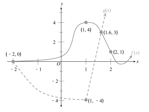


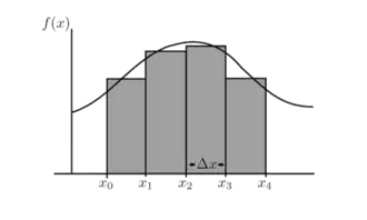

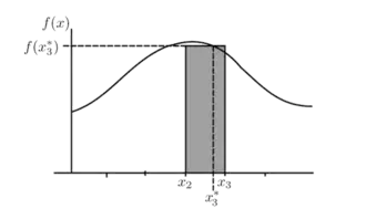


![{\displaystyle [x_{i-1},x_{i}]}](../_assets_/eb734a37dd21ce173a46342d1cc64c92/09cb12a889d47020c8ce7046a2eb60785e00c0b6.svg)


![{\displaystyle x_{i}^{*}\in [x_{i-1},x_{i}]}](../_assets_/eb734a37dd21ce173a46342d1cc64c92/dafeab86f1179399f11208ee27a15c76434aed3d.svg)

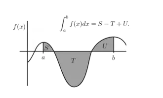


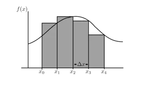
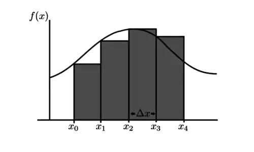


![{\displaystyle [0,1]}](../_assets_/eb734a37dd21ce173a46342d1cc64c92/738f7d23bb2d9642bab520020873cccbef49768d.svg)


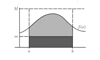


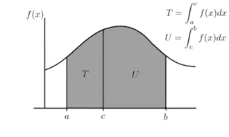


![{\displaystyle c\in [a,b]}](../_assets_/eb734a37dd21ce173a46342d1cc64c92/997256364b06acf0710e5d24da39e8c42991a249.svg)


![{\displaystyle x_{k}^{*}\in [a,b]}](../_assets_/eb734a37dd21ce173a46342d1cc64c92/3cbdda7ad947763ab5261e65436d0736bbe844b4.svg)


![{\displaystyle F(x)=\int \limits _{a}^{x}f(t)dt\quad {\text{for }}x\in [a,b]}](../_assets_/eb734a37dd21ce173a46342d1cc64c92/622d0ca08070b2d673bd8a757a67201a1619be8b.svg)


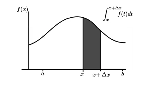


![{\displaystyle c\in [x,x+\Delta x]}](../_assets_/eb734a37dd21ce173a46342d1cc64c92/42b5053bab166c7c0f83e9c1d4096326f4a00df6.svg)


![{\displaystyle \lim _{\Delta x\to 0}{\Big [}x+\Delta x{\Big ]}=x\quad \Rightarrow \quad \lim _{\Delta x\to 0}c=x}](../_assets_/eb734a37dd21ce173a46342d1cc64c92/e3279e06d44cea4a17a91134775dec3e65e48a73.svg)


![{\displaystyle [a,\xi ]}](../_assets_/eb734a37dd21ce173a46342d1cc64c92/592a7dd205bdbcd1d8f67eca50eb6df3cadf5a22.svg)


![{\displaystyle 0\notin [a,b]}](../_assets_/eb734a37dd21ce173a46342d1cc64c92/a7e008e55b4d8c9220051749fbf4e809ee3e7d68.svg)


![{\displaystyle [4,9]}](../_assets_/eb734a37dd21ce173a46342d1cc64c92/7e52f81a7e0c9e3e24749e9b3a26c7236a25e302.svg)


![{\displaystyle \int \limits _{0}^{1}{\frac {dx}{x}}=\lim _{a\to 0^{+}}\left[\ln {\big (}|x|{\big )}{\Big |}_{a}^{1}\right]=\lim _{a\to 0^{+}}{\Big [}-\ln(a){\Big ]}}](../_assets_/eb734a37dd21ce173a46342d1cc64c92/57ed647eb635b1d7067bfbac60535b3b06f92cfa.svg)


![{\displaystyle {\begin{aligned}\int \limits _{-1}^{3}{\frac {dx}{x-2}}&=\lim _{b\to 2^{-}}\int \limits _{-1}^{b}{\frac {dx}{x-2}}+\lim _{a\to 2^{+}}\int \limits _{a}^{3}{\frac {dx}{x-2}}\\&=\lim _{b\to 2^{-}}\ln {\big (}|x-2|{\big )}{\Big |}_{-1}^{b}+\lim _{a\to 2^{+}}\ln {\big (}|x-2|{\big )}{\Big |}_{a}^{3}\\&=\lim _{b\to 2^{-}}{\Big [}\ln(2-b)-\ln(3){\Big ]}+\lim _{a\to 2^{+}}{\Big [}\ln(1)-\ln(a-2){\Big ]}\\&=\lim _{b\to 2^{-}}{\Big [}\ln(2-b){\Big ]}-\ln(3)+\lim _{a\to 2^{+}}{\Big [}-\ln(a-2){\Big ]}\\\end{aligned}}}](../_assets_/eb734a37dd21ce173a46342d1cc64c92/01e6267a1057ca0b7b0cffde3c0c3d14674f6fc2.svg)
![{\displaystyle \lim _{b\to 2^{-}}{\Big [}\ln(2-b){\Big ]}}](../_assets_/eb734a37dd21ce173a46342d1cc64c92/39478916ca0a1b49a263e2f24720b72e43da4ab3.svg)
![{\displaystyle \lim _{a\to 2^{+}}{\Big [}-\ln(a-2){\Big ]}}](../_assets_/eb734a37dd21ce173a46342d1cc64c92/0f8ee0057f0d7200b447f633a89a1e5e640ed0ff.svg)


![{\displaystyle \lim _{x\to \infty }{\Big [}x^{\frac {7}{2}}e^{-{\frac {x}{2}}}{\Big ]}=0}](../_assets_/eb734a37dd21ce173a46342d1cc64c92/a05363f54b8cc823ea4e40923318123e6ce4e80e.svg)


![{\displaystyle =\lim _{n\to \infty }\left[{\frac {b-a}{n}}\sum _{k=1}^{n}f(x_{k}^{*})\right]}](../_assets_/eb734a37dd21ce173a46342d1cc64c92/f40e7f31f18d3120cd5854df2694f3311235f55b.svg)


![{\displaystyle =\lim _{n\to \infty }\left[{\frac {b-a}{n}}\sum _{k=1}^{n}f{\big (}a+k{\tfrac {b-a}{n}}{\big )}\right]}](../_assets_/eb734a37dd21ce173a46342d1cc64c92/57b06290f59d25334cae6e3aed92ee16522f02e4.svg)

![{\displaystyle =\lim _{n\to \infty }\left[{\frac {2}{n}}\sum _{k=1}^{n}f{\big (}{\tfrac {2k}{n}}{\big )}\right]}](../_assets_/eb734a37dd21ce173a46342d1cc64c92/e8553f66ff312824e700fe689c3250cb6b09d949.svg)
![{\displaystyle =\lim _{n\to \infty }\left[{\frac {2}{n}}\sum _{k=1}^{n}\left({\frac {2k}{n}}\right)^{2}\right]}](../_assets_/eb734a37dd21ce173a46342d1cc64c92/1ce8f80fe79da631f23a6f06327f4de672f6612d.svg)
![{\displaystyle =\lim _{n\to \infty }\left[{\frac {2}{n}}\sum _{k=1}^{n}{\frac {4k^{2}}{n^{2}}}\right]}](../_assets_/eb734a37dd21ce173a46342d1cc64c92/0f54bd303d439fc7c9bcbd25f2722da50eb20115.svg)
![{\displaystyle =\lim _{n\to \infty }\left[{\frac {8}{n^{3}}}\sum _{k=1}^{n}k^{2}\right]}](../_assets_/eb734a37dd21ce173a46342d1cc64c92/eed134e3685881ee42d7a595d5f4f32286b053bf.svg)
![{\displaystyle =\lim _{n\to \infty }\left[{\frac {8}{n^{3}}}\cdot {\frac {n(n+1)(2n+1)}{6}}\right]}](../_assets_/eb734a37dd21ce173a46342d1cc64c92/e50443b6c2a1c7ab40b46665298d8ed1fd1f470c.svg)
![{\displaystyle =\lim _{n\to \infty }\left[{\frac {4}{3}}\cdot {\frac {2n^{2}+3n+1}{n^{2}}}\right]}](../_assets_/eb734a37dd21ce173a46342d1cc64c92/218c41740e24249292060210168ee62f21cdec64.svg)
![{\displaystyle =\lim _{n\to \infty }\left[{\frac {8}{3}}+{\frac {4}{n}}+{\frac {4}{3n^{2}}}\right]}](../_assets_/eb734a37dd21ce173a46342d1cc64c92/7a96db66ea4877d42fbf0c92253cb7b1be9c02b9.svg)

![{\displaystyle =\int \limits _{0}^{x}f(t)dt=\lim _{n\to \infty }\left[{\frac {x-0}{n}}\sum _{k=1}^{n}f(t_{k}^{*})\right]}](../_assets_/eb734a37dd21ce173a46342d1cc64c92/23b23ebc6e0ba82339f10e3faa642d16f27e931f.svg)
![{\displaystyle =\lim _{n\to \infty }\left[{\frac {x}{n}}\sum _{k=1}^{n}f{\big (}0+{\tfrac {k(x-0)}{n}}{\big )}\right]}](../_assets_/eb734a37dd21ce173a46342d1cc64c92/518c03c44547cc62f59e6c7eb03c8ff4837f181c.svg)
![{\displaystyle =\lim _{n\to \infty }\left[{\frac {x}{n}}\sum _{k=1}^{n}f{\big (}{\tfrac {kx}{n}}{\big )}\right]}](../_assets_/eb734a37dd21ce173a46342d1cc64c92/75b9da80feed61c6f9468e4035bb9842e475ee56.svg)

![{\displaystyle =\lim _{n\to \infty }\left[{\frac {x}{n}}\sum _{k=1}^{n}\left({\frac {kx}{n}}\right)^{2}\right]}](../_assets_/eb734a37dd21ce173a46342d1cc64c92/7c07b77821541c872c1ab8143e45e40a6bd106e1.svg)
![{\displaystyle =\lim _{n\to \infty }\left[{\frac {x}{n}}\sum _{k=1}^{n}{\frac {k^{2}\cdot x^{2}}{n^{2}}}\right]}](../_assets_/eb734a37dd21ce173a46342d1cc64c92/48139ada49a79ad9fde8058eaf5532f1cd5cab02.svg)
![{\displaystyle =\lim _{n\to \infty }\left[{\frac {x^{3}}{n^{3}}}\sum _{k=1}^{n}k^{2}\right]}](../_assets_/eb734a37dd21ce173a46342d1cc64c92/37d95b2b271bb3b4613e3da68589ab9ccb2e33e0.svg)
![{\displaystyle =\lim _{n\to \infty }\left[{\frac {x^{3}}{n^{3}}}\cdot {\frac {n(n+1)(2n+1)}{6}}\right]}](../_assets_/eb734a37dd21ce173a46342d1cc64c92/f8bb425da40536b03bad50620678a44fa8949b02.svg)
![{\displaystyle =\lim _{n\to \infty }\left[{\frac {x^{3}}{n^{3}}}\cdot {\frac {2n^{3}+3n^{2}+n}{6}}\right]}](../_assets_/eb734a37dd21ce173a46342d1cc64c92/736cb2ee176fb6a1b5aa882df8b6df53a270cf88.svg)
![{\displaystyle =x^{3}\cdot \lim _{n\to \infty }\left[{\frac {2n^{3}}{6n^{3}}}+{\frac {3n^{2}}{6n^{3}}}+{\frac {n}{6n^{3}}}\right]}](../_assets_/eb734a37dd21ce173a46342d1cc64c92/7e542a61937ccfd11fdfe054680a08e47f9ea8da.svg)
![{\displaystyle =x^{3}\cdot \lim _{n\to \infty }\left[{\frac {1}{3}}+{\frac {1}{2n}}+{\frac {1}{6n^{2}}}\right]}](../_assets_/eb734a37dd21ce173a46342d1cc64c92/e95f05d13bb1bdc37fa98d99ff8e5ea8e3b46997.svg)


![{\displaystyle {\frac {d[g(x)]}{dx}}=g'(x)}](../_assets_/eb734a37dd21ce173a46342d1cc64c92/e5fe744ba23aa86d2c675fbd3ec0e27851cb6526.svg)
![{\displaystyle dx={\frac {d[g(x)]}{g'(x)}}}](../_assets_/eb734a37dd21ce173a46342d1cc64c92/0336d72390fd9f03953ca0d3ba9f4fd2640f4f59.svg)

![{\displaystyle =\int g'(x)g(x)^{n}{\frac {d[g(x)]}{g'(x)}}}](../_assets_/eb734a37dd21ce173a46342d1cc64c92/8cd823ad23c038d62ad13fe29b7500cddc0bbbcc.svg)
![{\displaystyle =\int g(x)^{n}d[g(x)]}](../_assets_/eb734a37dd21ce173a46342d1cc64c92/97bc176225478964704055a4082c32a68afe1ddb.svg)


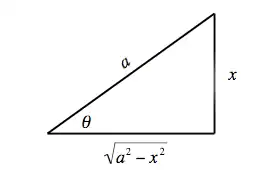


![{\displaystyle {\begin{aligned}\int \limits _{0}^{a}{\frac {1+x}{\sqrt {1-x^{2}}}}dx&=\int \limits _{0}^{\alpha }{\frac {1+\sin(\theta )}{\cos(\theta )}}\cos(\theta )d\theta &0<a<1\\&=\int \limits _{0}^{\alpha }{\bigl (}1+\sin(\theta ){\bigr )}d\theta &\alpha =\arcsin(a)\\&=\alpha +{\Big [}-\cos(\theta ){\Big ]}_{0}^{\alpha }\\&=\alpha +1-\cos(\alpha )\\&=1+\arcsin(a)-{\sqrt {1-a^{2}}}\end{aligned}}}](../_assets_/eb734a37dd21ce173a46342d1cc64c92/d34bea926b8fc779d11222829c812acd2aa7561a.svg)
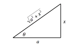


![{\displaystyle {\begin{aligned}\int \limits _{0}^{z}(x^{2}+a^{2})^{-{\frac {3}{2}}}dx&=a^{-2}\int \limits _{0}^{\alpha }\cos(\theta )d\theta &z>0\\&=a^{-2}{\Big [}\sin(\theta ){\Big ]}_{0}^{\alpha }&\alpha =\arctan \left({\tfrac {z}{a}}\right)\\&=a^{-2}\sin(\alpha )\\&=a^{-2}{\frac {\frac {z}{a}}{\sqrt {1+{\frac {z^{2}}{a^{2}}}}}}\\&={\frac {z}{a^{2}{\sqrt {a^{2}+z^{2}}}}}\end{aligned}}}](../_assets_/eb734a37dd21ce173a46342d1cc64c92/c4664e0be89a175f0c7b393341bd8ad28bbeb24c.svg)

![{\displaystyle {\begin{matrix}I&=&a^{2}\int _{0}^{\alpha }\sec ^{3}\theta \,d\theta &&&\alpha =\tan ^{-1}(z/a)\\&=&a^{2}\int _{0}^{\alpha }\sec \theta \,d\tan \theta &&&\\&=&a^{2}[\sec \theta \tan \theta ]_{0}^{\alpha }&-&a^{2}\int _{0}^{\alpha }\sec \theta \tan ^{2}\theta \,d\theta &\\&=&a^{2}\sec \alpha \tan \alpha &-&a^{2}\int _{0}^{\alpha }\sec ^{3}\theta \,d\theta &+a^{2}\int _{0}^{\alpha }\sec \theta \,d\theta \\&=&a^{2}\sec \alpha \tan \alpha &-&I&+a^{2}\int _{0}^{\alpha }\sec \theta \,d\theta \\\end{matrix}}}](../_assets_/eb734a37dd21ce173a46342d1cc64c92/313f2a452d4c096c9221cc6445317c894bb7eec0.svg)

![{\displaystyle ={\tfrac {a^{2}}{2}}{\Bigg (}\sec(\alpha )\tan(\alpha )+{\bigg [}\ln {\Big (}\sec(\theta )+\tan(\theta ){\Big )}{\bigg ]}_{0}^{\alpha }{\Bigg )}}](../_assets_/eb734a37dd21ce173a46342d1cc64c92/09ca73ab74b8a68988b561b211957b826c9bcc9f.svg)


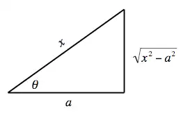


![{\displaystyle ={\bigg [}\tan(\theta )-\theta {\bigg ]}_{0}^{\alpha }\qquad \qquad \qquad \tan(\alpha )={\sqrt {\sec ^{2}(\alpha )-1}}}](../_assets_/eb734a37dd21ce173a46342d1cc64c92/eaf30ca894dfeaff2a765bb3ddb822a60753c656.svg)


![{\displaystyle =-{\bigg [}\tan(\theta )\cos(\theta ){\bigg ]}_{0}^{\alpha }+\int \limits _{0}^{\alpha }\sec(\theta )d\theta }](../_assets_/eb734a37dd21ce173a46342d1cc64c92/abddc762382184a13946dc8522620aa0ad23dff4.svg)
![{\displaystyle =-\sin(\alpha )+{\bigg [}\ln {\bigl (}\sec(\theta )+\tan(\theta ){\bigr )}{\bigg ]}_{0}^{\alpha }}](../_assets_/eb734a37dd21ce173a46342d1cc64c92/2b45d861d862f65be50d6cf40c62770494cfa763.svg)


![{\displaystyle {\begin{aligned}I&=\int \limits _{-1}^{1}{\frac {2-{\sqrt {2}}}{t^{2}+3-2{\sqrt {2}}}}dt+\int \limits _{-1}^{1}{\frac {2+{\sqrt {2}}}{t^{2}+3+2{\sqrt {2}}}}dt-\int \limits _{-1}^{1}{\frac {2}{1+t^{2}}}dt\\[8pt]&={\frac {4-2{\sqrt {2}}}{\sqrt {3-2{\sqrt {2}}}}}\cdot \arctan \left({\sqrt {3+2{\sqrt {2}}}}\right)+{\frac {4+2{\sqrt {2}}}{\sqrt {3+2{\sqrt {2}}}}}\cdot \arctan \left({\sqrt {3-2{\sqrt {2}}}}\right)-\pi \end{aligned}}}](../_assets_/eb734a37dd21ce173a46342d1cc64c92/07078edd3a9b891001284cfca52bce8ba80c3fe3.svg)


![{\displaystyle {\sqrt[{n}]{\frac {ax+b}{cx+d}}}}](../_assets_/eb734a37dd21ce173a46342d1cc64c92/e3e29101a1e02f716ce195ff15c28da35ee41746.svg)
![{\displaystyle u={\sqrt[{n}]{\frac {ax+b}{cx+d}}}}](../_assets_/eb734a37dd21ce173a46342d1cc64c92/85c6dab8107f08d3f4aff52530b7c762cc9923dc.svg)

![{\displaystyle \int {\frac {x}{\sqrt[{3}]{ax+b}}}\,dx}](../_assets_/eb734a37dd21ce173a46342d1cc64c92/8b50bc67a99e872f3a58779001d3a41029a4863f.svg)


![{\displaystyle Px+Q=p\cdot {\frac {d[ax^{2}+bx+c]}{dx}}+q}](../_assets_/eb734a37dd21ce173a46342d1cc64c92/55abfb79417c3bbfe85b1f296f5d748173d7e246.svg)


![{\displaystyle \int \limits _{a}^{b}f(x)dx\approx {\frac {b-a}{2n}}\left[f(x_{0})+2\sum _{i=1}^{n-1}{\bigl (}f(x_{i}){\bigr )}+f(x_{n})\right]={\frac {b-a}{2n}}{\bigg (}{f(x_{0})+2f(x_{1})+2f(x_{2})+\cdots +2f(x_{n-1})+f(x_{n})}{\bigg )}}](../_assets_/eb734a37dd21ce173a46342d1cc64c92/9f456afc1a77f39d5ce73e49bf7214e369357a2e.svg)
![{\displaystyle \approx {\frac {b-a}{6n}}\left[f(x_{0})+\sum _{i=1}^{n-1}\left((3-(-1)^{i})f(x_{i})\right)+f(x_{n})\right]}](../_assets_/eb734a37dd21ce173a46342d1cc64c92/3f5633de563d1a834994c89a7a28dfea9df98b30.svg)
![{\displaystyle ={\frac {b-a}{6n}}{\bigg [}f(x_{0})+4f{\bigl (}{\tfrac {x_{1}}{2}}{\bigr )}+2f(x_{1})+4f{\bigl (}{\tfrac {x_{3}}{2}}{\bigr )}+\cdots +4f{\bigl (}{\tfrac {x_{n-1}}{2}}{\bigr )}+f(x_{n}){\bigg ]}}](../_assets_/eb734a37dd21ce173a46342d1cc64c92/ed1d3402ef487bbd4d38b1236e31ee17be796480.svg)


![{\displaystyle {\bigl [}f(x_{i}^{*})-g(x_{i}^{*}){\bigr ]}\Delta x}](../_assets_/eb734a37dd21ce173a46342d1cc64c92/3efcbd6878b1c9c84285d7123766c63013ad35fe.svg)
![{\displaystyle A:=\sum _{i=1}^{n}{\Big [}f(x_{i}^{*})-g(x_{i}^{*}){\Big ]}\Delta x}](../_assets_/eb734a37dd21ce173a46342d1cc64c92/b532cb175e18edf6dc343ec2abc5acbf183415b7.svg)
![{\displaystyle A=\lim _{n\to \infty }\sum _{i=1}^{n}{\Big [}f(x_{i}^{*})-g(x_{i}^{*}){\Big ]}\Delta x}](../_assets_/eb734a37dd21ce173a46342d1cc64c92/66f6dd23a75bdf922a3a92f28772310ab80f2805.svg)


![{\displaystyle [c,d]}](../_assets_/eb734a37dd21ce173a46342d1cc64c92/d85b3b21d6d891d97f85e263d394e3c90287586f.svg)


![{\displaystyle A:=\sum _{i=1}^{n}{\Big [}f(y_{i}^{*})-g(y_{i}^{*}){\Big ]}\Delta y}](../_assets_/eb734a37dd21ce173a46342d1cc64c92/8670a382efc3d742ae073ca7fc9f2f77fda78423.svg)
![{\displaystyle A=\lim _{n\to \infty }\sum _{i=1}^{n}{\Big [}f(y_{i}^{*})-g(y_{i}^{*}){\Big ]}\Delta y}](../_assets_/eb734a37dd21ce173a46342d1cc64c92/9682357a788e80bae02a003b2ac2a10beb6bbc1a.svg)

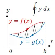


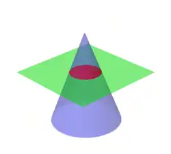


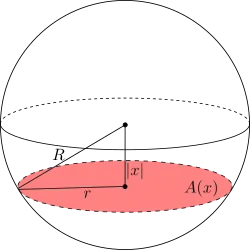


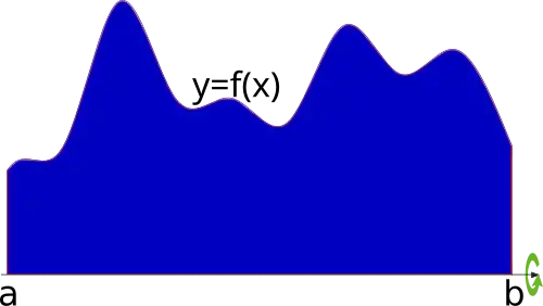


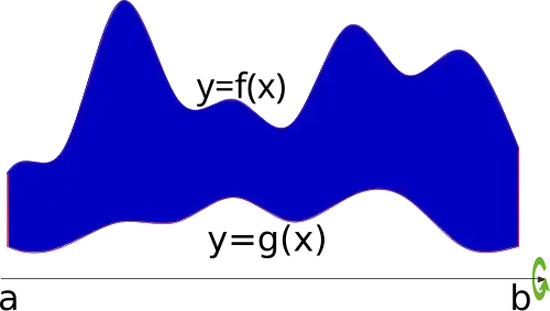
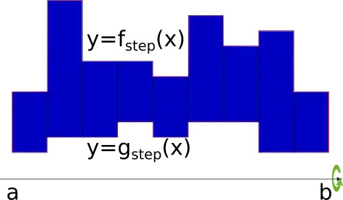


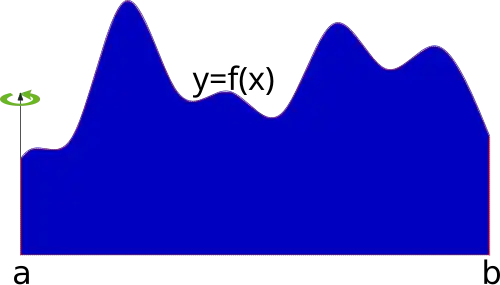


![{\displaystyle {\frac {d}{dt}}\left[{\frac {dy}{dx}}\right]={\frac {\frac {d^{2}y}{dx}}{dt}}}](../_assets_/eb734a37dd21ce173a46342d1cc64c92/0198c905950f907fc395629a80df9e52a848aa87.svg)


![{\displaystyle {\frac {d}{dt}}\left[{\frac {dy}{dx}}\right]\times {\frac {dt}{dx}}}](../_assets_/eb734a37dd21ce173a46342d1cc64c92/ca571f86c1822cf3d98fe25e50455b4fef266548.svg)
![{\displaystyle {\frac {d}{dt}}[\csc(t)]\times \cos(t)=-\csc ^{2}(t)\times \cos(t)}](../_assets_/eb734a37dd21ce173a46342d1cc64c92/e7c99782726e6ac69d97a09443d606b1e3d7719c.svg)


![{\displaystyle [\alpha ,\beta ]}](../_assets_/eb734a37dd21ce173a46342d1cc64c92/878fce9eb3ba664f0ad4d025f04214fa85ee9583.svg)


![{\displaystyle [0,R]}](../_assets_/eb734a37dd21ce173a46342d1cc64c92/3ea1a7293db142452ce72c16d8f7c427fccf434c.svg)


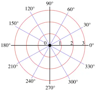
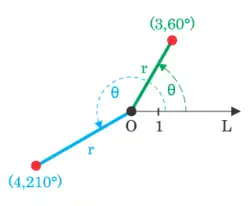


![{\displaystyle (-180^{\circ },180^{\circ }]}](../_assets_/eb734a37dd21ce173a46342d1cc64c92/52564e11cb8ecd24997d7929ef3ff9a87052b335.svg)

![{\displaystyle (-\pi ,\pi ]}](../_assets_/eb734a37dd21ce173a46342d1cc64c92/7fbb1843079a9df3d3bbcce3249bb2599790de9c.svg)

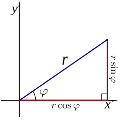


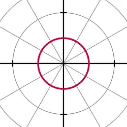


.PNG)


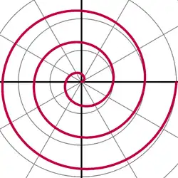


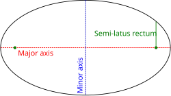


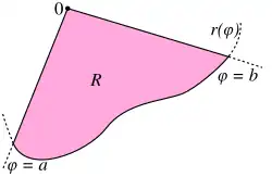


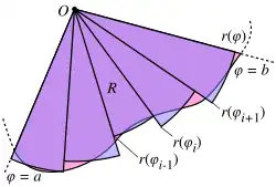


![{\displaystyle {\begin{aligned}2\int \limits _{-1}^{1}{\sqrt {1-x^{2}}}dx&=2\left[{\frac {\arcsin(x)+x{\sqrt {1-x^{2}}}}{2}}\right]_{-1}^{1}\\&=\arcsin(1)-\arcsin(-1)\\&=\pi \end{aligned}}}](../_assets_/eb734a37dd21ce173a46342d1cc64c92/06ab5a1b76940c74774887b8beda9c6dc2874db0.svg)


![{\displaystyle \int \limits _{0}^{2\pi }\int \limits _{0}^{1}r\,dr\,d\theta =\int \limits _{0}^{2\pi }\left[{\frac {r^{2}}{2}}\right]_{0}^{1}d\theta =\int \limits _{0}^{2\pi }{\frac {d\theta }{2}}=\left[{\frac {\theta }{2}}\right]_{0}^{2\pi }={\frac {2\pi }{2}}=\pi }](../_assets_/eb734a37dd21ce173a46342d1cc64c92/848eb50f444342ee1abaab37bf6f0fbf83633f52.svg)


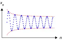


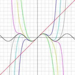 sin(x) and Taylor approximations, polynomials of degree 1, 3, 5, 7, 9, 11 and 13.


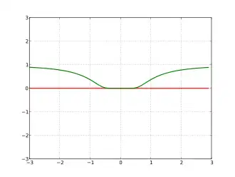 The function is not analytic: the Taylor series is 0, although the function is not.


![{\displaystyle {\frac {d}{dx}}\left[\sum _{n=0}^{\infty }a_{n}x^{n}\right]=\sum _{n=0}^{\infty }a_{n+1}(n+1)(x-c)^{n}}](../_assets_/eb734a37dd21ce173a46342d1cc64c92/26a350f64b58c17f29063a5641a5254c611512a1.svg)