OpenSCAD User Manual/Transformations
Basic concept
Transformations affect their child nodes and as the name implies transform them in various ways such as moving, rotating or scaling the child. Transformations are written before the object they affect e.g.
translate([10,20,30])
    cube(10);
Notice that there is no semicolon following transformation command. Transformations can be applied to a group of child nodes by using '{' and '}' to enclose the subtree e.g.
translate([0,0,-5])
{
    cube(10);
    cylinder(r=5,h=10);
}
Cascading transformations are used to apply a variety of transforms to a final child. Cascading is achieved by nesting statements e.g.
rotate([45,45,45])
    translate([10,20,30])
        cube(10);
Combining transformations is a sequential process, going from right to left. Consider the following two transformations:
color("red")   translate([0,10,0])  rotate([45,0,0])     cube(5);
color("green") rotate([45,0,0])     translate([0,10,0])  cube(5);
While these contain the same operations, the first rotates a cube around the origin and then moves it by the offset specified for the translate, before finally coloring it red. By contrast, the second sequence first moves a cube, and then rotates it around the origin, before coloring it green. In this case the rotation causes the cube to move along an arc centered at the origin. The radius of this arc is the distance from the origin, which was set by the preceding translation. The different ordering of the rotate and translate transformations causes the cubes to end up in different places.
Advanced concept
As OpenSCAD uses different libraries to implement capabilities this can introduce some inconsistencies to the F5 preview behaviour of transformations. Traditional transforms (translate, rotate, scale, mirror & multimatrix) are performed using OpenGL in preview, while other more advanced transforms, such as resize, perform a CGAL operation, behaving like a CSG operation affecting the underlying object, not just transforming it. In particular this can affect the display of modifier characters, specifically "#" and "%", where the highlight may not display intuitively, such as highlighting the pre-resized object, but highlighting the post-scaled object.
scale
Scales its child elements using the specified vector. Note that unlike the resize transformation below, this is multiplicative, so the current size is multiplied by the factor provided in the vector. The argument name is optional.
Usage Example:
scale(v = [x, y, z]) { ... }
cube(10);
translate([15,0,0]) scale([0.5,1,2]) cube(10);
_example.JPG)
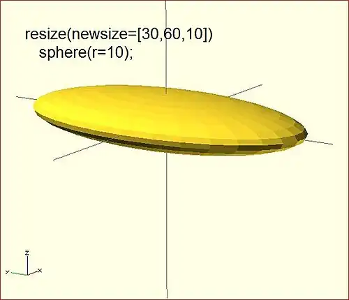
resize
Modifies the size of the child object to match the given x,y, and z sizes.
resize() is a CGAL operation, and like others such as render() operates with full geometry, so even in preview this takes time to process.
Usage Example:
// resize the sphere to extend 30 in x, 60 in y, and 10 in the z directions.
resize(newsize=[30,60,10]) sphere(r=10);
If x,y, or z is 0 then that dimension is left as-is.
// resize the 1x1x1 cube to 2x2x1
resize([2,2,0]) cube();
If the 'auto' parameter is set to true, it auto-scales any 0-dimensions to match. For example.
// resize the 1x2x0.5 cube to 7x14x3.5
resize([7,0,0], auto=true) cube([1,2,0.5]);
The 'auto' parameter can also be used if you only wish to auto-scale a single dimension, and leave the other as-is.
// resize to 10x8x1. Note that the z dimension is left alone.
resize([10,0,0], auto=[true,true,false]) cube([5,4,1]);
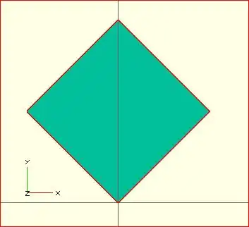
rotate
Rotates its child 'a' degrees about the axis of the coordinate system or around an arbitrary axis. The argument names are optional if the arguments are given in the same order as specified.
//Usage:
rotate(a = deg_a, v = [x, y, z]) { ... }
// or
rotate(deg_a, [x, y, z]) { ... }
rotate(a = [deg_x, deg_y, deg_z]) { ... }
rotate([deg_x, deg_y, deg_z]) { ... }
The 'a' argument (deg_a) can be an array, as expressed in the later usage above; when deg_a is an array, the 'v' argument is ignored. Where 'a' specifies multiple axes then the rotation is applied in the following order: x then y then z. That means the code:
rotate(a=[ax,ay,az]) {...}
is equivalent to:
rotate(a=[0,0,az]) rotate(a=[0,ay,0]) rotate(a=[ax,0,0]) {...}
For example, to flip an object upside-down, you can rotate your object 180 degrees around the 'y' axis.
rotate(a=[0,180,0]) { ... }
This is frequently simplified to
rotate([0,180,0]) { ... }
The optional argument 'v' is a vector that determines an arbitrary axis about which the object is rotated.
When specifying a single axis the 'v' argument allows you to specify which axis is the basis for rotation. For example, the equivalent to the above, to rotate just around y
rotate(a=180, v=[0,1,0]) { ... }
When specifying a single axis, 'v' is a vector defining an arbitrary axis for rotation; this is different from the multiple axis above. For example, rotate your object 45 degrees around the axis defined by the vector [1,1,0],
rotate(a=45, v=[1,1,0]) { ... }
_example.JPG)
Rotate with a single scalar argument rotates around the Z axis. This is useful in 2D contexts where that is the only axis for rotation. For example:
rotate(45) square(10);
Rotation rule help

For the case of:
rotate([a, b, c]) { ... };
"a" is a rotation about the X axis, from the +Y axis, toward the +Z axis.
"b" is a rotation about the Y axis, from the +Z axis, toward the +X axis.
"c" is a rotation about the Z axis, from the +X axis, toward the +Y axis.
These are all cases of the Right Hand Rule. Point your right thumb along the positive axis, your fingers show the direction of rotation.
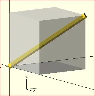
Thus if "a" is fixed to zero, and "b" and "c" are manipulated appropriately, this is the spherical coordinate system.
So, to construct a cylinder from the origin to some other point (x,y,z):
x= 10; y = 10; z = 10; // point coordinates of end of cylinder

length = norm([x,y,z]);  // radial distance
b = acos(z/length); // inclination angle
c = atan2(y,x);     // azimuthal angle

rotate([0, b, c])
    cylinder(h=length, r=0.5);
%cube([x,y,z]); // corner of cube should coincide with end of cylinder
// Griglia woofer 20cm - OpenSCAD // Specifiche: // outer_dia = 199 mm (leggermente ridotto per tolleranze stampante) // plate_thickness = 5 mm // ring_width = 15 mm (anello esterno pieno) // hex_circ_dia = 50 mm (esagoni) // hex_flat_to_flat = 50 // hex_radius = hex_circ_dia/2 // margin from inner hex area to ring inner edge = 1 mm // bolt_circle = 170 mm, 4 boccole affogate (Ø esterno 6 mm, depth 5 mm) // back lip: depth 5 mm, radial thickness 2 mm
$fn = 64; // qualità per cerchi (puoi aumentare o diminuire)
// // PARAMETERS // outer_dia = 199; plate_thickness = 5; ring_width = 15; hex_circ_dia = 50; hex_r = hex_circ_dia/2; // distance from center to vertex (circumradius) hex_flat = hex_circ_dia; // flat-to-flat margin = 1; // gap between hex pattern extent and inner edge of ring bolt_circle = 170; n_bolts = 4; boccola_outer_d = 6; boccola_depth = 5; boccola_counter_from_front = 0; // 0 = countersunk from front face into plate back_lip_depth = 5; back_lip_thickness = 2; // radial thickness of lip
// Derived outer_r = outer_dia/2; inner_r = outer_r - ring_width; // radius of inner edge of ring where hexagons start hex_max_r = inner_r - margin; // max radius within which hex centers/vertices must fit
module hexagon(center=[0,0], side = hex_r) {
   // flat-top hexagon (side = circumradius)
   pts = [];
   for (i = [0:5]) {
       a = i*60; // degrees
       x = center[0] + side * cos(a);
       y = center[1] + side * sin(a);
       pts = concat(pts, x,y);
   }
   polygon(points = pts);
}
module hex_grid() {
   // flat-top hex spacing
   s = hex_r;
   hex_h = sqrt(3) * s; // vertical span of hex
   x_step = 1.5 * s;
   y_step = hex_h;
   // start from negative extents
   x_min = -hex_max_r;
   x_max = hex_max_r;
   y_min = -hex_max_r;
   y_max = hex_max_r;
   col = 0;
   x = x_min;
   for (col = 0; x <= x_max + 0.001; x = x + x_step, col = col + 1) {
       y_offset = (col % 2 == 0) ? 0 : y_step/2;
       y = y_min - y_step + y_offset;
       for (; y <= y_max + 0.001; y = y + y_step) {
           // compute vertices and check if all inside hex_max_r
           ok = true;
           for (i = [0:5]) {
               a = i*60;
               vx = x + s * cos(a);
               vy = y + s * sin(a);
               if (sqrt(vx*vx + vy*vy) > hex_max_r + 0.0001) ok = false;
           }
           if (ok) {
               translate([x, y, 0]) linear_extrude(height = plate_thickness + 1) // extra to ensure full cut
                   hexagon([0,0], s);
           }
       }
   }
}
// alloggi boccole: boss cilindrico che verrà sottratto (cut) dal volume per creare la sede module boccola_at_angle(angle_deg) {
   ang = angle_deg;
   bx = cos(ang) * (bolt_circle/2);
   by = sin(ang) * (bolt_circle/2);
   translate([bx, by, 0])
       rotate([0,0,0])
           cylinder(r = boccola_outer_d/2, h = boccola_depth + 1, $fn=64);
}
// OUTER SHAPE module grille_body() {
   // main plate: big disk
   difference() {
       // base plate (with slight extra thickness for boolean reliability)
       translate([0,0,0])
           cylinder(r = outer_r, h = plate_thickness, $fn=128);
       // subtract hex pattern (through hole)
       hex_grid();
       // subtract bolt holes (clearance)
       for (i = [0: n_bolts-1]) {
           ang = -90 + i * (360 / n_bolts); // start at -90 deg so first at top
           translate([cos(ang)*(bolt_circle/2), sin(ang)*(bolt_circle/2), 0])
               cylinder(r = (boccola_outer_d/2) + 0.5, h = plate_thickness+1, $fn=64);
       }
       // subtract inner open area within inner_r to create ring-only perimeter
       translate([0,0,0])
           cylinder(r = inner_r, h = plate_thickness + 2, $fn=128);
   }
}
// back lip (battuta) - a ring that sits behind (negative Z) module back_lip() {
   // annular ring: from outer_r - back_lip_thickness_in_radial to inner_r + ? adjust so lip only at ring portion
   lip_outer_r = outer_r;
   lip_inner_r = inner_r; // lip matches inner edge of ring
   translate([0,0,-back_lip_depth]) difference() {
       // big ring
       union() {
           cylinder(r = lip_outer_r, h = back_lip_depth, $fn=128);
           // keep inner hole
       }
       translate([0,0,-0.1])
           cylinder(r = lip_inner_r, h = back_lip_depth + 0.2, $fn=128);
       // subtract screw holes inside lip so screws can go through lip if necessary
       for (i = [0: n_bolts-1]) {
           ang = -90 + i * (360 / n_bolts);
           translate([cos(ang)*(bolt_circle/2), sin(ang)*(bolt_circle/2), -back_lip_depth])
               cylinder(r = (boccola_outer_d/2)+0.2, h = back_lip_depth + 2, $fn=64);
       }
   }
}
// boccole affogate: create countersinks/pockets on the FRONT face so che la vite autofilettante si infili module countersunk_boccole() {
   for (i = [0: n_bolts-1]) {
       ang = -90 + i * (360 / n_bolts);
       translate([cos(ang)*(bolt_circle/2), sin(ang)*(bolt_circle/2), 0])
           // shallow cylindrical pocket from front into plate
           cylinder(r = boccola_outer_d/2 + 0.2, h = boccola_depth, $fn=64);
   }
}
// Build final model: union of grille body + back lip, then subtract countersunk pockets & hex holes already subtracted in grille_body difference() {
   union() {
       grille_body();
       back_lip();
   }
   // subtract the countersunk pockets from front (so that they are open holes)
   countersunk_boccole();
}
cube(2,center = true);
translate([5,0,0])
   sphere(1,center = true);
_example.JPG)
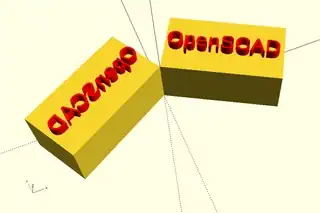
mirror
Transforms the child element to a mirror of the original, as if it were the mirror image seen through a plane intersecting the origin. The argument to mirror() is the normal vector of the origin-intersecting mirror plane used, meaning the vector coming perpendicularly out of the plane. Each coordinate of the original object is altered such that it becomes equidistant on the other side of this plane from the closest point on the plane. For example, mirror([1,0,0]), corresponding to a normal vector pointing in the x-axis direction, produces an object such that all positive x coordinates become negative x coordinates, and all negative x coordinates become positive x coordinates.
Function signature:
mirror(v= [x, y, z] ) { ... }
Examples
The original is on the right side. Note that mirror doesn't make a copy. Like rotate and scale, it changes the object.
-
![hand(); // original mirror([1,0,0]) hand();](../_assets_/0c70a452f799bfe840676ee341124611/Mirror-x.png)
hand(); // originalmirror([1,0,0]) hand(); -
![hand(); // original mirror([1,1,0]) hand();](../_assets_/0c70a452f799bfe840676ee341124611/Mirror-x-y.png)
hand(); // originalmirror([1,1,0]) hand(); -
![hand(); // original mirror([1,1,1]) hand();](../_assets_/0c70a452f799bfe840676ee341124611/Mirror-x-y-z.png)
hand(); // originalmirror([1,1,1]) hand();
 // original
 rotate([0,0,-30]){
   cube([23,12,10]);
   translate([0.5, 4.4, 9.9]){
     color("red", 1.0){
       linear_extrude(height=2){
         text("OpenSCAD", size= 3);
       }
     }
   }
 }
 // mirrored
 mirror([1,0,0]){
   rotate([0,0,-30]){
     cube([23,12,10]);
     translate([0.5, 4.4, 9.9]){
       color("red", 1.0){
         linear_extrude(height=2){
           text("OpenSCAD", size= 3);
         }
       }
     }
   }
 }
multmatrix
Multiplies the geometry of all child elements with the given affine transformation matrix, where the matrix is 4×3 - a vector of 3 row vectors with 4 elements each, or a 4×4 matrix with the 4th row always forced to [0,0,0,1].
Usage: multmatrix(m = [...]) { ... }
This is a breakdown of what you can do with the independent elements in the matrix (for the first three rows):
| Scale X | Shear X along Y | Shear X along Z | Translate X |
| Shear Y along X | Scale Y | Shear Y along Z | Translate Y |
| Shear Z along X | Shear Z along Y | Scale Z | Translate Z |
The fourth row is forced to [0,0,0,1] and can be omitted unless you are combining matrices before passing to multmatrix, as it is not processed in OpenSCAD. Each matrix operates on the points of the given geometry as if each vertex is a 4 element vector consisting of a 3D vector with an implicit 1 as its 4th element, such as v=[x, y, z, 1]. The role of the implicit fourth row of m is to preserve the implicit 1 in the 4th element of the vectors, permitting the translations to work. The operation of multmatrix therefore performs m*v for each vertex v. Any elements (other than the 4th row) not specified in m are treated as zeros.
This example rotates by 45 degrees in the XY plane and translates by [10,20,30], i.e. the same as translate([10,20,30]) rotate([0,0,45]) would do.
angle=45;
multmatrix(m = [ [cos(angle), -sin(angle), 0, 10],
                 [sin(angle),  cos(angle), 0, 20],
                 [         0,           0, 1, 30],
                 [         0,           0, 0,  1]
              ]) union() {
   cylinder(r=10.0,h=10,center=false);
   cube(size=[10,10,10],center=false);
}
The following example demonstrates combining affine transformation matrices by matrix multiplication, producing in the final version a transformation equivalent to rotate([0, -35, 0]) translate([40, 0, 0]) Obj();. Note that the signs on the sin function appear to be in a different order than the above example, because the positive one must be ordered as x into y, y into z, z into x for the rotation angles to correspond to rotation about the other axis in a right-handed coordinate system.
module Obj() {
   cylinder(r=10.0,h=10,center=false);
   cube(size=[10,10,10],center=false);
}

// This itterates into the future 6 times and demonstrates how multimatrix is moving the object around the center point
for(time = [0 : 15 : 90]){
    y_ang=-time;
    mrot_y = [ [ cos(y_ang), 0,  sin(y_ang), 0],
               [         0,  1,           0, 0],
               [-sin(y_ang), 0,  cos(y_ang), 0],
               [         0,  0,           0, 1]
             ];
    mtrans_x = [ [1, 0, 0, 40],
                 [0, 1, 0,  0],
                 [0, 0, 1,  0],
                 [0, 0, 0,  1]
               ];

    echo(mrot_y*mtrans_x);

    // This is the object at [0,0,0]
    Obj();

    // This is the starting object at the [40,0,0] coordinate
    multmatrix(mtrans_x) Obj();

    // This is the one rotating and appears 6 times
    multmatrix(mrot_y * mtrans_x) Obj();
};
This example skews a model, which is not possible with the other transformations.
M = [ [ 1  , 0  , 0  , 0   ],
      [ 0  , 1  , 0.7, 0   ],  // The "0.7" is the skew value; pushed along the y axis as z changes.
      [ 0  , 0  , 1  , 0   ],
      [ 0  , 0  , 0  , 1   ] ] ;
multmatrix(M) {  union() {
    cylinder(r=10.0,h=10,center=false);
    cube(size=[10,10,10],center=false);
} }
This example shows how a vector is transformed with a multmatrix vector, like this all points in a point array (polygon) can be transformed sequentially. Vector (v) is transformed with a rotation matrix (m), resulting in a new vector (vtrans) which is now rotated and is moving the cube along a circular path radius=v around the z axis without rotating the cube.
angle=45;
 m=[
        [cos(angle), -sin(angle), 0, 0],
        [sin(angle),  cos(angle), 0, 0],
        [         0,           0, 1, 0]
   ];

v=[10,0,0];
vm=concat(v,[1]); // need to add [1]
vtrans=m*vm;
echo(vtrans);
translate(vtrans)cube();
More?
Learn more about it here:
color
Displays the child elements using the specified RGB color + alpha value. This is only used for the F5 preview as CGAL and STL (F6) do not currently support color. The alpha value defaults to 1.0 (opaque) if not specified.
Function signature:
color( c = [r, g, b, a] ) { ... }
color( c = [r, g, b], alpha = 1.0 ) { ... }
color( "#hexvalue" ) { ... }
color( "colorname", 1.0 ) { ... }
Note that all four values for red, green, blue, and alpha (RGBA) are expected to be written as floating point values in the range [0.0:1.0].
Graphics industry common practice is to specify RGBA values as integers in the range [0:255].
To convert values from 0 to 256 to the range needed for the color module they can be individually scaled, or the color vector may be scaled thus: color([0,125,255]/255) { ... }
![]() Warning: Transparent shapes should be drawn into the scene after opaque ones to be sure that the latter are visible through transparent shapes that are "in front" of them.
If drawn after a solid object behind a transparent one might not be visible.
Issue #1390 is about this issue.
Warning: Transparent shapes should be drawn into the scene after opaque ones to be sure that the latter are visible through transparent shapes that are "in front" of them.
If drawn after a solid object behind a transparent one might not be visible.
Issue #1390 is about this issue.
Using Named Colors
[Note: Requires version 2011.12]
Colors can be specified by name in a case insensitive string.
For example color("red") sphere(5); will color the sphere red.
Alpha may be given as a second parameter: color("Blue",0.5) cube(5); or by name color("green",alpha=0.5) cube(5);.
The color values on the list all have their alpha value set to 1.0, thus fully opaque.
The available color names are taken from the World Wide Web Consortium's SVG color list. Expand the following section for the chart of the color names. OpenSCAD adds an additional named color, "transparent", with this RGBA value, [0,0,0,0], making it a 100% transparent black.
(note that both spellings of grey or gray are accepted, so slategrey and slategray both work):
|
|
|
|
| |||||||||||||||||||||||||||||||||||||||||||||||||||||||||||||||||||||||||||||||||||||||||||||||||||||||||||||||||||||||||||||||||||||||||||||||||||||||||
Using Hexcode Colors
[Note: Requires version 2019.05] Hex values are given as a string of hexadecimal digits, in either RGB or RGBA format, meaning either as three or four values, and each value may be given as one or two hexadecimal digits:
#rgb#rgba#rrggbb#rrggbbaa
If the alpha value is included in the hex value and also as separate parameter, the separate parameter takes precedence.
Example
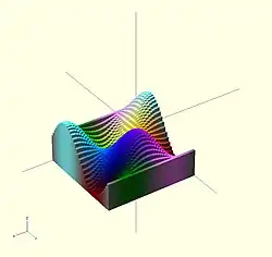
Here's a code fragment that draws a wavy multicolor object
  for(i=[0:36]) {
    for(j=[0:36]) {
      color( [0.5+sin(10*i)/2, 0.5+sin(10*j)/2, 0.5+sin(10*(i+j))/2] )
      translate( [i, j, 0] )
      cube( size = [1, 1, 11+10*cos(10*i)*sin(10*j)] );
    }
  }
Being that -1<=sin(x)<=1 then 0<=(1/2 + sin(x)/2)<=1 , allowing for the RGB components assigned to color to remain within the [0,1] interval.
Example 2
In cases where you want to optionally set a color based on a parameter you can use the following trick:
 module myModule(withColors=false) {
    c=withColors?"red":undef;
    color(c) circle(r=10);
 }
Setting the colorname to undef keeps the default colors.
offset
[Note: Requires version 2015.03]
default with no argument at all is (r = 1, chamfer = false)
radius takes precedence if both r and delta are given.
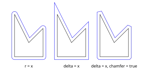
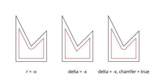
Offset generates a new 2d interior or exterior outline from an existing outline. There are two modes of operation: radial and delta.
- The radial method creates a new outline as if a circle of some radius is rotated around the exterior (r > 0) or interior (r < 0) of the original outline.
- The delta method creates a new outline with sides having a fixed distance outward (delta > 0) or inward (delta < 0) from the original outline.
The construction methods produce an outline that is either inside or outside of the original outline. For outlines using delta, when the outline goes around a corner, it can be given an optional chamfer.
Offset is useful for making thin walls by subtracting a negative-offset construction from the original, or the original from a positive offset construction.
Offset can be used to simulate some common solid modeling operations:
- Fillet:
offset(r=-3) offset(delta=+3)rounds all inside (concave) corners, and leaves flat walls unchanged. However, holes less than 2*r in diameter vanish. - Round:
offset(r=+3) offset(delta=-3)rounds all outside (convex) corners, and leaves flat walls unchanged. However, walls less than 2*r thick vanish.
- Parameters
The first parameter may be passed without a name, in which case it is treated as the r parameter below. All other parameters must be named if used.
r or delta
- Number. Amount to offset the polygon. When negative, the polygon is offset inward.
- r (default parameter if not named) specifies the radius of the circle that is rotated about the outline, either inside or outside. This mode produces rounded corners. The name may be omitted; that is,
offset(c)is equivalent tooffset(r=c). - delta specifies the distance of the new outline from the original outline, and therefore reproduces angled corners. No inward perimeter is generated in places where the perimeter would cross itself.
- r (default parameter if not named) specifies the radius of the circle that is rotated about the outline, either inside or outside. This mode produces rounded corners. The name may be omitted; that is,
- chamfer
- Boolean. (default false) When using the delta parameter, this flag defines if edges should be chamfered (cut off with a straight line) or not (extended to their intersection). This parameter has no effect on radial offsets.
$fa, $fs, and $fn
- The circle resolution special variables may be used to control the smoothness or facet size of curves generated by radial offsets. They have no effect on delta offsets.
Examples
// Example 1

linear_extrude(height = 60, twist = 90, slices = 60) {
   difference() {
     offset(r = 10) {
      square(20, center = true);
     }
     offset(r = 8) {
       square(20, center = true);
     }
   }
 }
// Example 2

module fillet(r) {
   offset(r = -r) {
     offset(delta = r) {
       children();
     }
   }
}
fill
[Note: Requires version Development snapshot]
Fill removes holes from polygons without changing the outline. For convex polygons the result is identical to hull().
Examples

// Example 1

t = "OpenSCAD";

linear_extrude(15) {
	text(t, 50);
}
color("darkslategray") {
	linear_extrude(2) {
		offset(4) {
			fill() {
				text(t, 50);
			}
		}
	}
}
minkowski
Displays the minkowski sum of child nodes.
Usage example:
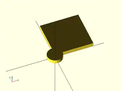
Say you have a flat box, and you want a rounded edge. There are multiple ways to do this (for example, see hull below), but minkowski is elegant. Take your box, and a cylinder:
 $fn=50;
 cube([10,10,1]);
 cylinder(r=2,h=1);
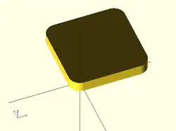
Then, do a minkowski sum of them (note that the outer dimensions of the box are now 10+2+2 = 14 units by 14 units by 2 units high as the heights of the objects are summed):
$fn=50;
minkowski()
{
  cube([10,10,1]);
  cylinder(r=2,h=1);
}
NB: The origin of the second object is used for the addition. The following minkowski sums are different: the first expands the original cube by +1 in -x, +x, -y, +y from cylinder, expand 0.5 units in both -z, +z from cylinder. The second expands it by +1 in -x, +x, -y, +y and +z from cylinder, but expand 0 in the -z from cylinder.
minkowski() {
	cube([10, 10, 1]);
	cylinder(1, center=true);
}
minkowski() {
	cube([10, 10, 1]);
	cylinder(1);
}
Warning: for high values of $fn the minkowski sum may end up consuming lots of CPU and memory, since it has to combine every child node of each element with all the nodes of each other element. So if for example $fn=100 and you combine two cylinders, then it does not just perform 200 operations as with two independent cylinders, but 100*100 = 10000 operations.
Warning: if one of the inputs is compound, such as:
    {
         translate([0, 0, collar])
         sphere(ball);
         cylinder(collar, ball, ball);
    }
it may be treated as two separate inputs, resulting in an output which is too large, and has features between surfaces that should be unaltered with respect to one another. If so, use union().
hull
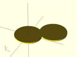
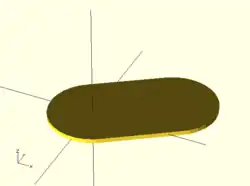
Displays the convex hull of child nodes.
Usage example:
hull() {
    translate([15,10,0]) circle(10);
    circle(10);
}
The Hull of 2D objects uses their projections (shadows) on the xy plane, and produces a result on the xy plane. Their Z-height is not used in the operation.
Referring to the illustration of a convex hull of two cylinders, it is computationally more efficient to use hull() on two 2D circles and linear_extrude the resulting 2D shape into a 3D shape, rather than using hull() on two cylinders, even though the resulting object appears identical. Complex geometries involving hull() can be rendered faster by starting out in 2D, if possible.